Chapter 7
(AST301) Design and Analysis of Experiments II
7 Blocking and Confounding in the \(2^k\) factorial design
7.1 Introduction
Blocking is a technique for dealing with controllable nuisance variables
Two cases are considered
Replicated designs
Unreplicated designs
7.2 Blocking a replicated \(2^k\) factorial design
In many situations, it is impossible to perform all the runs in a \(2^k\) factorial experiment under homogeneous conditions.
The design technique used in these situations is blocking.
Consider \(2^k\) design with \(n\) replicates, but \(n2^k\) homogeneous experimental units are not available.
If blocks of size \(2^k\) are available, we can run this experiment in \(n\) blocks.
The method of analyzing the factorial design, where each replicate is run in one of the blocks, has already been discussed (in Chapter 5)
Experimental units are randomly assigned to treatments within each block.
EXAMPLE 7.1
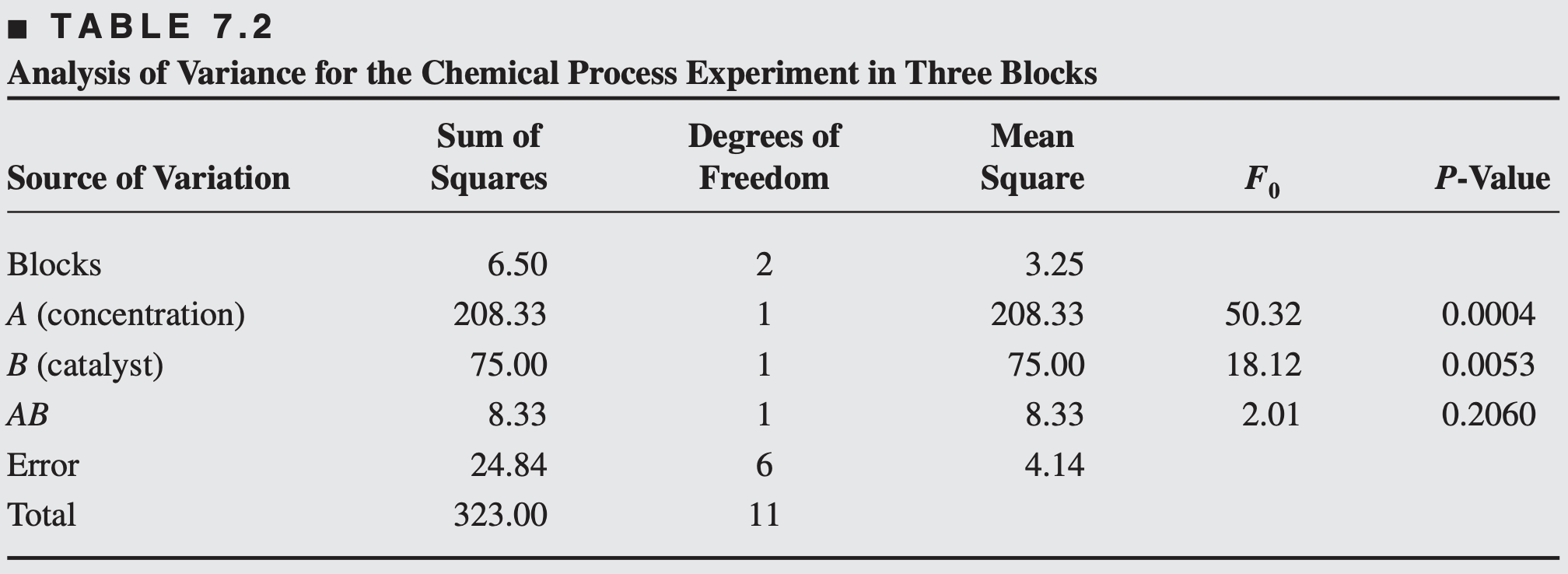
Consider the chemical process experiment described in Section 6.2
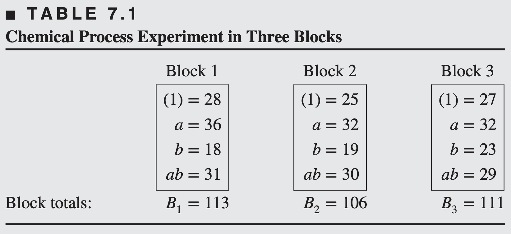
Suppose that only four experimental trials can be made from a single batch of raw material.
Therefore, three batches of raw material will be required to run all three replicates of this design.
Table 7.1 shows the design, where each batch of raw material corresponds to a block.
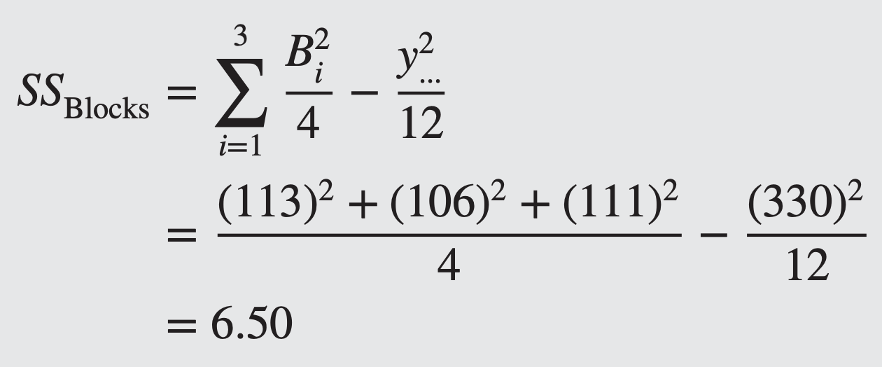
- This is the “usual” method of calculating a block sum of squares

7.3 Confounding \(2^k\) factorial design
In many problems, it is impossible to perform a complete replicate of factorial design in one block.
Confounding is a design technique for arranging a complete factorial experiment in blocks, where block size is smaller than the number of treatment combinations in one replicate.
This technique causes information about certain treatment effects (usually high-order interactions) to be confounded with blocks (or indistinguishable from blocks)
The designs are incomplete block design, but the special structure of the \(2^k\) factorial system allows us a simplified method of analysis.
Confounding \(2^k\) factorial design in 2 blocks
Suppose we want to run a single replicate of a \(2^2\) design. Four treatment combinations require a quantity of raw materials, but the raw material is only large enough for two treatment combinations to be tested.
So two batches of raw materials are required and if batches of raw materials are considered as blocks then we need to assign two treatment combinations to each block.
One possible design for this problem
\[ \begin{array}{cc} \hline \text{Block 1} & \text{Block 2} \\ \hline \\ (1) & a \\ ab & b \\ \hline \end{array} \]
Order of the treatment combinations run within blocks are randomly determined, and also randomly decide which block is to run first.
\[ \begin{array}{cc} \hline \text{Block 1} & \text{Block 2} \\ \hline \\ (1) & a \\ ab & b \\ \hline \end{array} \]
Block effect is the difference of the average response of two blocks, i.e. \([ab - a -b + (1)]/2\)
Estimates of other effects \[\begin{align*} A&=[ab + a - b - (1)]/2\\ B&=[ab - a + b - (1)]/2 \\ AB&=[ab - a - b + (1)]/2 \end{align*}\]
The contrasts of the treatment combinations of \(AB\) and block effects are the same, i.e. \(AB\) is confounded with blocks.
If (1) and \(b\) had been assigned to block 1 and \(a\) and \(ab\) to block 2, the main effect \(A\) would have been confounded with blocks.
The usual practice is to confound the highest order interaction with blocks.
There are different methods of constructing blocks, the simplest one is based on the plus-minus signs of the factorial design.
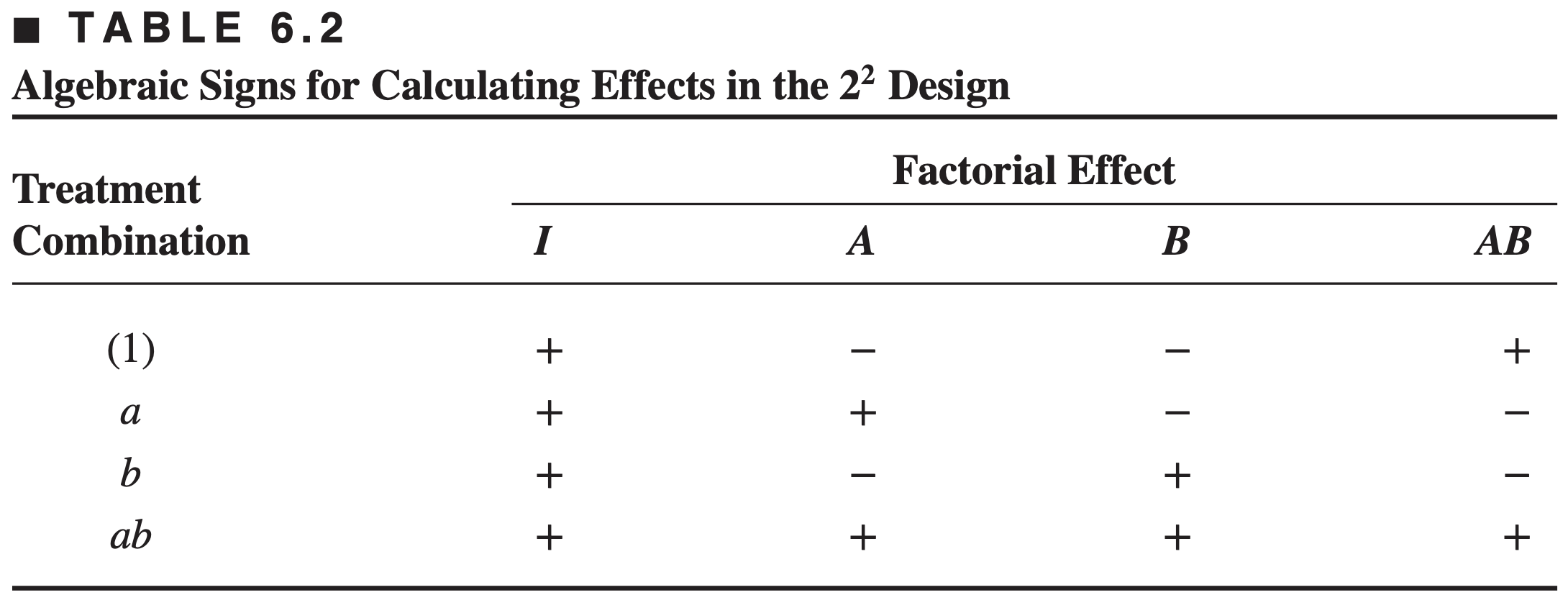
- Treatment combinations of the blocks are determined by the signs of the of the \(AB\) effects, where
- \((1)\) and \(ab\) with plus signs are assigned to “block 1”
- \(a\) and \(b\) with minus signs are assigned to “block 2”
For this design \(AB\) is confounded with blocks.
This scheme can be used to confound any \(2^k\) design in two blocks.
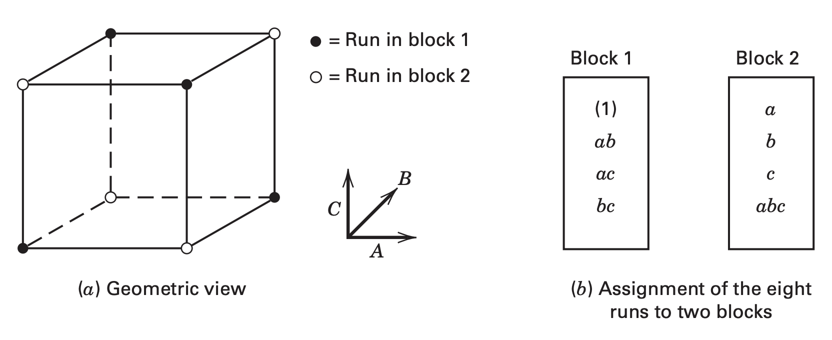
As a second example, consider a \(2^3\) design run in two blocks.
Suppose we wish to confound the three-factor interaction \(ABC\) with blocks.
From the table of plus and minus signs for \(2^3\) design (Table 7.4, p.313), we assign the treatment combinations that are minus on \(ABC\) to block 1 and those that are plus on \(ABC\) to block 2.
The resulting design is shown in the following figure.
Other Methods for Constructing the Blocks
The second method of constructing blocks for \(2^k\) design uses the linear combination (known as defining contrast) \[\begin{align*} L&=\alpha_1 x_1 + \alpha_2 x_2 + \cdots + \alpha_k x_k, \end{align*}\] where \(x_i\) is the level of the \(ith\) factor appearing in a particular treatment combination and \(\alpha_i\) is the exponent appearing in the effect to be confounded.
For the \(2^k\) design, both \(\alpha_i\) and \(x_i\) will take values either 0 or 1
For the \(2^2\) design, if \(AB\) is the treatment combination of interest then \(L=x_1 + x_2\), where both \(\alpha\)’s are 1.
The defining contrast \[\begin{align*} L&=\alpha_1 x_1 + \alpha_2 x_2 + \cdots + \alpha_k x_k \end{align*}\] becomes \(L=x_1 + x_2\) for the treatment combination \(AB\) (effect to be confounded).
First find the values of \(L\) for different effect of \(2^2\) design: \[\begin{align*} (1) : \; L= 0 + 0 &=0\\ a : \; L= 1 + 0 & =1 \\ b : \; L= 0 + 1 & =1 \\ ab : \; L= 1 + 1 & =2 \end{align*}\]
The defining contrast \(L=x_1 + x_2\) for the treatment combination \(AB\) (effect to be confounded).
First find the values of \(L\) for different effect of \(2^2\) design: \[\begin{align*} \left.\begin{array}{cc} (1) : \; L= 0 + 0 &=0\\ a : \; L= 1 + 0 & =1 \\ b : \; L= 0 + 1 & =1 \\ ab : \; L= 1 + 1 & =2 \end{array}\right\}\Rightarrow \left\{\begin{array}{rl} (1) : \; L= 0 + 0 &=0\; (\text{mod 2})\\ a : \; L= 1 + 0 & =1 \; (\text{mod 2})\\ b : \; L= 0 + 1 & =1 \; (\text{mod 2})\\ ab : \; L= 1 + 1 & ={\color{purple}\bf 0} \; (\text{mod 2}) \end{array}\right. \end{align*}\]
- Treatment combinations that produce the same value of \(L\)~(mod 2) will be placed in the same block
- In this case, \(\{(1), ab\}\) will be placed in one block and \(\{a, b\}\) in the other block.
Exercise:
Find the blocks if you want to run a \(2^3\) design in 2 blocks with ABC confounded with blocks.
Third method
The third method of constructing blocks for \(2^k\) design is based on the principal block, the block that contains the treatment combination \((1)\).
The treatment combinations of the principal block have a useful group-theoretic property
- they form a group with respect to multiplication modulus 2, i.e. treatment combinations of principal block, except \((1)\), can be obtained by multiplying any two treatment combinations of the principal block.
- treatment combinations in the other block (or blocks) may be generated by multiplying one element in the new block by the each element in the principal block (mod 2).
Consider the \(2^3\) design where \(ABC\) is the effect to be confounded (corresponding defining contrast \(L=x_1 + x_2 + x_3\))
The principal block consists of the treatment combinations {\(\{(1), ab, ac, bc\}\)} and it can be shown \[\begin{align*} {\color{blue}ab\cdot ac =a^2bc =bc},\; {\color{magenta}ab\cdot bc=ab^2c=ac},\;{\color{gray}ac\cdot bc=abc^2=ab} \end{align*}\]
Treatment combinations of other blocks can be generated as (since we know that \(b\) is in the other block) \[\begin{align*} {\color{blue}b\cdot (1)=b}, \;\;\;&{\color{magenta}b\cdot ab=ab^2=a}\\ {\color{blue}b\cdot ac=abc}, \;\;\;&{\color{magenta}b\cdot bc=b^2c=c} \end{align*}\] So, the elements of the second block are {\(\{a, b, c, abc\}\)}.
Assignment of eight runs in two blocks: \[\begin{align*} \text{Block I}:&\;\; \{(1), ab, ac, bc\} \\ \text{Block II}:&\;\; \{a, b, c, abc\} \end{align*}\]
Estimation of error
When the number of factors is small, the experiment needs to replicate to obtain an estimate of error.
When the number of factors is large, one can ignore the higher-order interactions and can get the estimate of error.
7.4 Confounding \(2^k\) factorial design in 4 blocks
We have seen:
- Constructing \(2^2\) designs confounded in 2 blocks of 2 observations, or in general
- constructing \(2^k\) designs confounded in 2 blocks of \(2^{k-1}\) observations
New topic: constructing \(2^k\) designs confounded in 4 blocks of \(2^{k-2}\) observations
These designs are useful in situations where the number of factors is relatively large (e.g. \(k\geq 4\)), and block sizes are relatively small.
The general procedure for constructing a \(2^k\) design confounded in four blocks is to choose two effects to generate the blocks, automatically confounding a third effect that is the generalized interaction of the first two.
The design is constructed by using the two defining contrasts (L1, L2) and the group-theoretic properties of the principal block.
In selecting effects to be confounded with blocks, care must be exercised to obtain a design that does not confound effects that may be of interest.
For example, in a \(2^5\) design we might choose to confound \(ABCDE\) and \(ABD\), which automatically confounds \(CE\), an effect that is probably of interest.
A better choice is to confound \(ADE\) and \(BCE\), which automatically confounds \(ABCD\).
Suppose the interest is to construct a single replication of \(2^5\) design where each of the four blocks will have only 8 runs.
Construction of this design requires selection of two effects to be confounded with blocks, say \(ADE\) and \(BCE\). The corresponding defining contrasts are \[\begin{align*} L_1 & = x_1 + x_4 + x_5 \\ L_2 & = x_2 + x_3 + x_5. \end{align*}\] Treatment combinations are assigned to different blocks by the values of \(L_1\) (mod 2) and \(L_2\) (mod 2), e.g. treatments with \[\begin{align*} (L_1=0, \; L_2=0)\longrightarrow \text{``Block 1''}\\ (L_1=1, \;L_2=0)\longrightarrow \text{``Block 2''}\\ (L_1=1, \;L_2=0)\longrightarrow \text{``Block 3''}\\ (L_1=1, L_2=1)\longrightarrow \text{``Block 4''}. \end{align*}\]
Defining contrasts corresponding to treatment combinations \(ADE\) and \(BCE\) to be confounded with blocks are \[\begin{align*} L_1 & = x_1 + x_4 + x_5 \\ L_2 & = x_2 + x_3 + x_5. \end{align*}\] Allocation of treatment combinations to different blocks \[\begin{align*} L_1=0, L_2=0&\;\; \text{for}\;\;{\color{blue}(1), ad, bc, abcd, abe, bde, ace, cde}\\ L_1=1, L_2=0&\;\; \text{for}\;\;{\color{purple} a, d, abc, bcd, be, abde, ce, acde}\\ L_1=0, L_2=1&\;\; \text{for}\;\;{\color{green}c, acd, b, abd, abce, bcde, ae, ade}\\ L_1=1, L_2=1&\;\; \text{for}\;\;{\color{gray}e, ade, bce, abcde, ab, bd, ac, cd } \end{align*}\]
Example
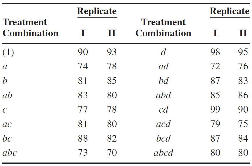
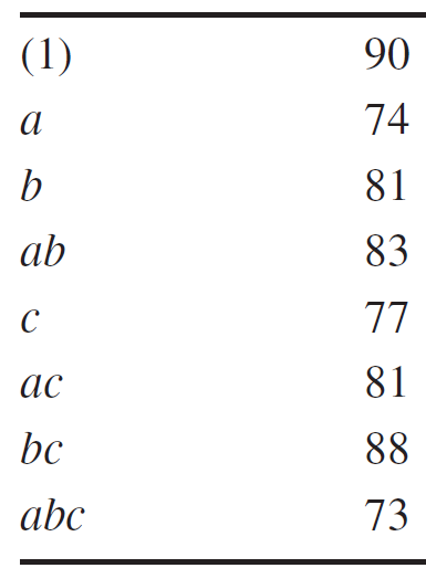
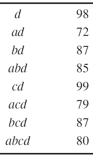
An experiment was performed to improve the yield of a chemical process. Four factors were selected. A design is constructed with four blocks of four observations each with ABD and ABC confounded (and consequently CD) with blocks. The results are shown in the following table. Analyze the data.
7.5 Confounding \(2^k\) factorial design in \(2^p\) blocks
Confounding the \(2^{k}\) factorial design in four blocks can be extended to the construction of a \(2^{{k}}\) factorial design confounded in \(2^p\) blocks \((p<k)\), where each block contains exactly \(2^{k-p}\) runs.
We select \(p\) independent effects to be confounded, where by “independent” we mean that no effect chosen is the generalized interaction of the others.
The blocks may be generated by use of the \(p\) defining contrasts \({L}_1, L_2, \ldots, {L_p}\) associated with these effects.
In addition, exactly \(2^p-{p}-1\) other effects will be confounded with blocks, these being the generalized interactions of those \({p}\) independent effects initially chosen.
Care should be exercised in selecting effects to be confounded so that information on effects that may be of potential interest is not sacrificed.
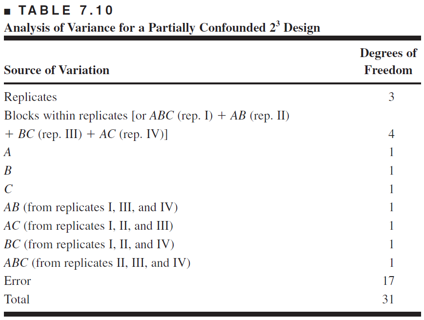
The statistical analysis of these designs is straightforward. Sums of squares for all the effects are computed as if no blocking had occurred.
Then, the block sum of squares is found by adding the sums of squares for all the effects confounded with blocks.
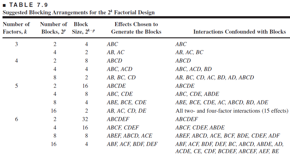
Suppose we wish to construct a \(2^6\) design confounded in \(2^3=8\) blocks of \(2^3=8\) runs each.
Table \(7.9\) indicates that we would choose \(ABEF\), \({ABCD}\), and \({ACE}\) as the \({p}=3\) independent effects to generate the blocks.
The remaining \(2^p-p-1=2^3-3-1=4\) effects that are confounded are the generalized interactions of these three; that is, \[ \begin{aligned} (A B E F)(A B C D) & =A^2 B^2 C D E F=C D E F \\ (A B E F)(A C E) & =A^2 B C E^2 F=B C F \\ (A B C D)(A C E) & =A^2 B C^2 E D=B D E \\ (A B E F)(A B C D)(A C E) & =A^3 B^2 C^2 D E^2 F=A D F \end{aligned} \]
7.6 Partial Confounding
- Unless experimenters have a prior estimate of error or are willing to assume certain interactions to be negligible, they must replicate the design to obtain an estimate of error.

The above figure shows a \(2^3\) factorial in two blocks with ABC confounded, replicated four times.
Information on the ABC interaction cannot be retrieved for a two blocks \(2^3\) factorial design with ABC confounded, because ABC is confounde with blocks in each replicate. This design is said to be completely confounded.
- Consider the \(2^3\) design given below where ABC is confounded in replicate I, \(AB\) is confounded in replicate II, \(BC\) is confounded in replicate III, and \(AC\) is confounded in replicate IV.

As a result, information on \(ABC\) can be obtained from replicates II, III, and IV; information on \(AB\) can be obtained from replicates I, III, and IV; information on \(AC\) can be obtained from replicates I, II, and III; and information on \(BC\) can be obtained from replicates I, II, and IV.
Three-quarters information can be obtained on the interactions because they are unconfounded in only three replicates. This design is said to be partially confounded.
Example 7.3
Consider Example 6.1, in which an experiment was conducted to develop a plasma etching process. There were three factors, \(A=\) gap, \(B=\) gas flow, and \(C=R F\) power, and the response variable is the etch rate.
Suppose that only four treatment combinations can be tested during a shift, and because there could be shift-to-shift differences in etching tool performance, the experimenters decide to use shifts as a blocking factor.
Thus, each replicate of the \(2^3\) design must be run in two blocks. Two replicates are run, with \(A B C\) confounded in replicate I and \(A B\) confounded in replicate II. The data are as follows:
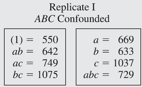
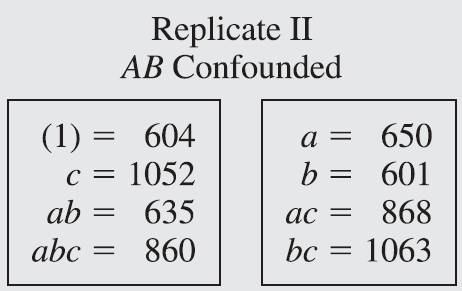
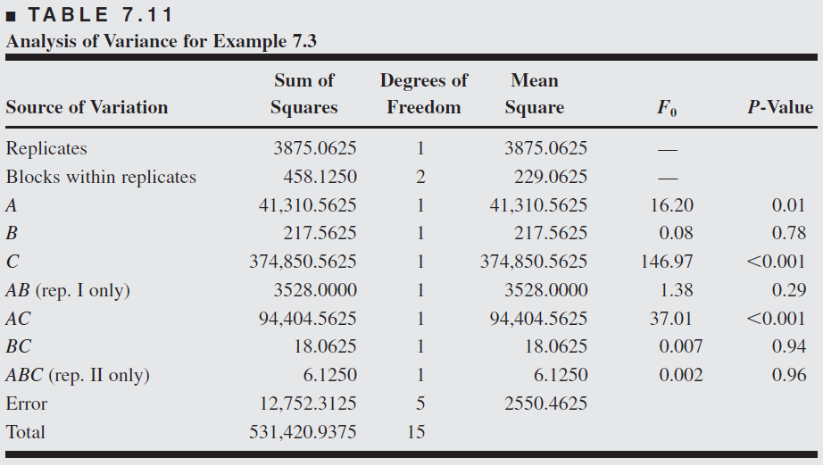
The sums of squares for \(A, B, C, A C\), and \(B C\) may be calculated in the usual manner, using all 16 observations.
However, we must find \(S S_{A B C}\) using only the data in replicate II and \(S S_{A B}\) using only the data in replicate I as follows:


where \(R_h\) is the total of the observations in the \(h\)th replicate.
The block sum of squares would be \(S S_{\text {Blocks }}=458.1250\), which is the sum of
- \(S S_{A B C}\) from replicate I and
- \(S S_{A B}\) from replicate II,
The analysis of variance is summarized in Table 7.11. The main effects of \(A\) and \(C\) and the \(A C\) interaction are important.
Example
An experiment was performed to improve the yield of a chemical process. Four factors were selected, and two replicates of a completely randomized experiment were run.
The results are shown in the following table. Suppose that ABCD was confounded in replicate I and ABC was confounded in replicate II. Perform the statistical analysis of this design.
