Chapter 9

(AST301) Design and Analysis of Experiments II

9 Additional Design and Analysis Topics for Factorial and Fractional Factorial Designs

9.1 The $3^k$ Factorial Design

• The three-level design is written as a $3^k$ factorial design. It means that $k$ factors are considered, each at 3 levels.

• These are (usually) referred to as low, intermediate and high levels. These levels are numerically expressed as 0, 1, and 2.

• One could have considered the digits -1, 0, and +1, but this may be confusing with respect to the 2-level designs since 0 is reserved for center points. Therefore, we will use the 0, 1, 2 scheme.

• A third level for a continuous factor facilitates investigation of a quadratic relationship between the response and each of the factors.

---

• Each treatment combination in the $3^k$ design is denoted by $k$ digits, where the first digit indicates the level of factor $A$, the second digit indicates the level of factor $B,\dots$, and the $k$th digit indicates the level of factor $K$.

• For example, in a $3^2$ design, 00 denotes the treatment combination corresponding to $A$ and $B$ both at the low level, and 01 denotes the treatment combination corresponding to $A$ at the low level and $B$ at the intermediate level.

---

• In the $3^k$ system of designs, when the factors are quantitative, we often denote the low, intermediate, and high levels by $-1,0$, and $+1$, respectively. This facilitates fitting a regression model relating the response to the factor levels.

• Regression model for analyzing $3^2$ factorial design $$y={\beta }_0+{\beta }_1{x}_1+{\beta }_2{x}_2+{\beta }_{12}{x}_1{x}_2+{\beta }_{11}{x}_1^2+{\beta }_{22}{x}^2$$

---

• The $3^k$ design is useful when curvature of the response surface is concerned, however, there are more useful methods for examining curvature of response surface than the $3^k$ design, which are

  • response surface design
  • $2^k$ design with center points (central composite design)

The $3^2$ Design

The $3^2$ design has two factors, each at three levels. There are $3^2=9$ treatment combinations and there are 8 degrees of freedom between these treatment combinations: $$000102101112202122$$

• Main effect of $A$: 2 degrees of freedom
• Main effect of $B$: 2 degrees of freedom
• Interaction $AB$: 4 degrees of freedom

For $n$ replicates, there are $3^{2}n-1$ total degrees of freedom and $3^2(n-1)$ degrees of freedom for error

The sums of squares for the effects $A$, $B$, and $AB$ can be computed by usual methods discussed in Chapter 5.

---

The two degrees of freedom of each main effect can be represented by a linear and a quadratic component each with a single degrees of freedom. Suppose that both factors $A$ and $B$ are quantitative

The two-factor interaction $AB$ can be partitioned into two ways:

1. Dividing $AB$ into four single-degrees-of-freedom components $$A{B}_{L\times L},A{B}_{L\times Q},A{B}_{Q\times L},A{B}_{Q\times Q}$$ This can be done by fitting the terms ${\beta }_{12}{x}_1{x}_2$, ${\beta }_{122}{x}_1{x_2}^2,{}_2,{\beta }_{112}{x}_1^2{x}_2$ and,${\beta }_{1122}{x}^2{}_1{x}_2^2$ respectively.

2. The second method is based on the orthogonal Latin squares. Two Latin squares are said to be orthogonal if one square is superimposed on the other, produce all possible ordered pairs of symbols exactly once.

Example 5.5

The effective life of a cutting tool installed in a numerically controlled machine is thought to be affected by the cutting speed and the tool angle. Three speeds and three angles are selected, and a $3^2$ factorial experiment with two replicates is performed. The coded data are shown below

---

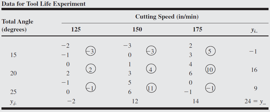
Since the factors are quantitative, and both factors have three levels, a second-order model such as $$\begin{array}{rl}& y={\beta }_0+{\beta }_1{x}_1+{\beta }_2{x}_2+{\beta }_{12}{x}_1{x}_2+{\beta }_{11}{x}^2{}_1+{\beta }_{22}{x}_2^2+{\beta }_{122}{x}_1{x}_2^2+\\ & {\beta }_{112}{x}^2{}_1{x}_2+{\beta }_{1122}{x}_1^2{x}_2^2\end{array}$$ can be fit to the data.

From the data we obtain sum of squares as $${AB}_{L\times L}=8,{AB}_{L\times Q}=42.67,{AB}_{Q\times L}=2.67\text{ and }{AB}_{Q\times Q}=8$$ That is ${SS}_{AB}=8+42.67+2.67+8=61.34$.

---

The second method is based on orthogonal Latin squares. This method does not require that the factors be quantitative, and it is usually associated with the case where all factors are qualitative.

The two factors $A$ and $B$ correspond to the rows and columns, respectively, of a $3\times 3$ Latin square.

For the above example, two particular $3\times 3$ Latin squares are shown superimposed on the cell totals below:

---

Treatment combination totals from Example 5.5 with two orthogonal Latin squares superimposed

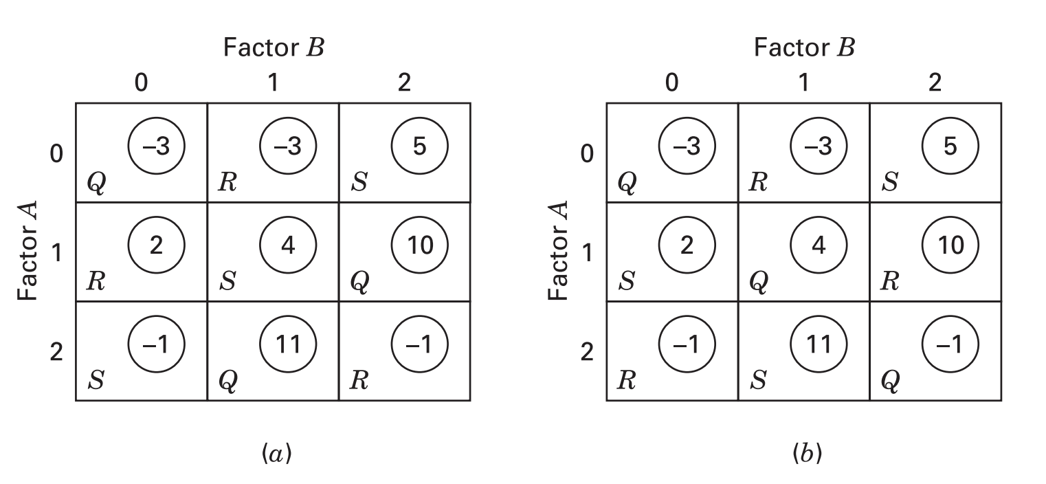
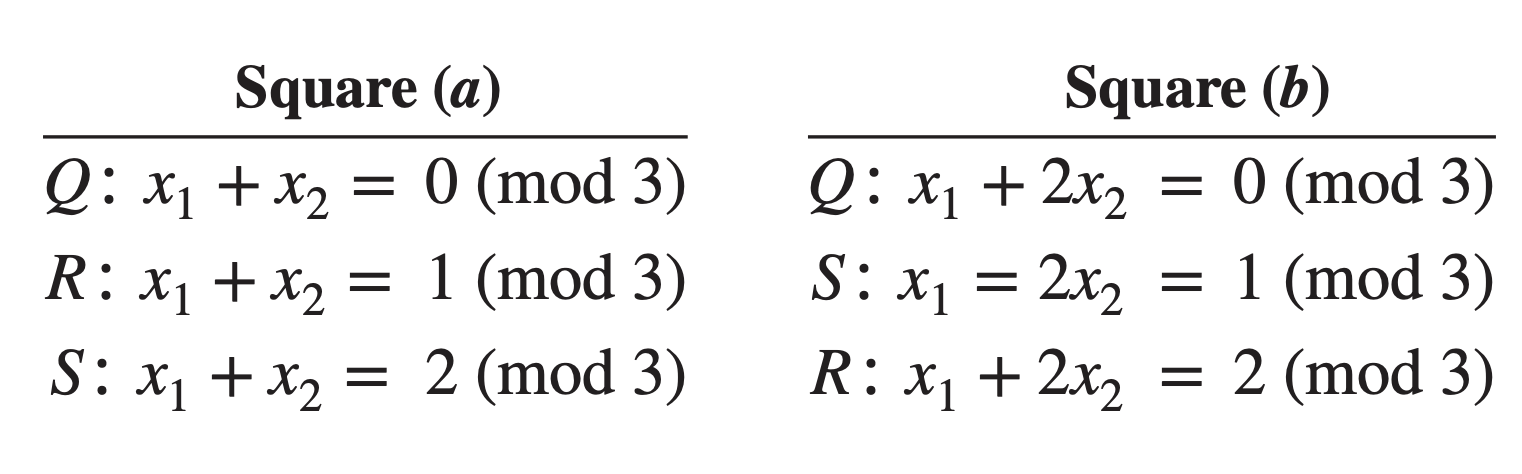
So, SS from first table is known as $AB$ component of the interaction, and SS from the second table is known as $A{B}^2$ component of the interaction

---

Total of the letters from the first table: $Q=18,R=-2,S=8$. Sum of squares between these totals is 33.3 with 2 df.

Total of the letters from the second table: $Q=0,R=6,S=18$. Sum of squares between these totals is 28 with 2 df.

$S{S}_{AB}=33.3+28=61.3$ with 4 df

It can also be shown that $A{B}^2=(A{B}^2{)}^2=A^2{B}^4=A^{2}B$

---

There is another way of calculating the $AB$ and $A{B}^2$ components of the interaction:

Add the data by diagonals downward from the left to right and the totals are $$\begin{array}{ll}-3+4-1& =0\\ -3+10-1& =6\\ 5+2+11& =18\end{array}\}\Rightarrow \text{sum of squares of these totals}=28=A{B}^2$$

Add the data by diagonals downward from the right to left and the totals are $$\begin{array}{ll}5+4-1& =8\\ -3+2-1& =-2\\ -3+11+10& =18\end{array}\}\Rightarrow \text{sum of squares of these totals}=33.3=AB$$

---

Yates called these components of interaction as the $I$ and $J$ components of interaction: $$\begin{array}{rl}I(AB)=& A{B}^2\\ J(AB)=& AB\end{array}$$

The $3^3$ design

The $3^3$ design has three factors $(A,B,C)$, each has three levels and there $3^3=27$ treatment combinations

Among 26 degrees of freedom, 6 for the main effects, 12 for the two-factor interactions, and 8 for the three-factor interaction

For $n$ replicates, there are $3^{3}n-1$ total degrees of freedom and $3^3(n-1)$ degrees of freedom for error

---

Sums of squares can be calculated using the standard methods, in addition to that, if the factors are quantitative

• Main effects can be partitioned into linear $(L)$ and quadratic $(Q)$ components, each with one degrees of freedom
• Two-factor interactions can be partitioned into components corresponding to $L\times L$, $L\times Q$, $Q\times L$, $Q\times Q$
• Three-factor interaction can be partitioned into components corresponding to $L\times L\times L$, $L\times L\times Q$, etc.

---

The sum of squares corresponding to the two-factor interaction has $I$ and $J$ components, e.g. $I(AB)=A{B}^2$ and $J(AB)=AB$

The sum of squares corresponding to a three-factor interaction has $W$, $X$, $Y$, and $Z$ components, e.g.
$$\begin{array}{rl}W(ABC)& =A{B}^2{C}^2,X(ABC)=AB{C}^2,\\ Y(ABC)& =A{B}^{2}C,Z(ABC)=ABC\end{array}$$

The general $3^k$ design

The $3^k$ factorial design has $k$ factors, each has 3 levels, so there are $3^k$ treatment combinations with $3^k-1$ degrees of freedom between them

There are

• $k$ main effects, each has 2 degrees of freedom
• $(\genfrac{}{}{0ex}{}{k}{2})$ two-factor interactions, each has $2^2=4$ degrees of freedom
• one $k$-factor interaction, which has $2^k$ degrees of freedom

If there are $n$ replications then total degrees of freedom will be $n{3}^k-1$ and error degrees of freedom is $3^k(n-1)$

Sums of squares for different effects are computed by usual method of factorial design

---

Any $h$-factor interaction has $2^{h-1}$ orthogonal components, each of which has 2 degrees of freedom

E.g. The four-factor interaction $ABCD$ has $2^{4-1}=8$ orthogonal components, which are $$\begin{array}{rlrlrlr}ABC{D}^2& & AB{C}^{2}D& & A{B}^{2}CD& & ABCD\\ AB{C}^2{D}^2& & A{B}^{2}C{D}^2& & A{B}^2{C}^{2}D& & A{B}^2{C}^2{D}^2\end{array}$$

Note that only exponent allowed for the first letter is 1 and if the exponent of the first letter is not 1 then the entire expression must be squared, e.g.
$$\begin{array}{r}{A}^{2}BCD=(A^{2}BCD{)}^2=A^4{B}^2{C}^2{D}^2=A{B}^2{C}^2{D}^2\end{array}$$

These interaction components have no physical meaning but they are useful in constructing more complex designs

9.2 Confounding in the $3^k$ Factorial Design

Even when a single replicate of the $3^k$ design is considered, the design requires so many runs that it is unlikely that all $3^k$ runs can be made under uniform conditions.

Thus, confounding in blocks is often necessary. The $3^k$ design may be confounded in $3^p$ incomplete blocks, where $p<k$.

Thus, these designs may be confounded in three blocks, nine blocks, and so on.

The $3^k$ factorial design in three blocks

The three blocks have two degrees of freedom, so there must be two degrees of freedom confounded with blocks

In the $3^k$ factorial design

• each main effect has two degrees of freedom
• each two-factor interaction has four degrees of freedom, which can be decomposed into two components (e.g. $AB$ and $A{B}^2$), each of which has two degrees of freedom
• each three-factor interaction has eight degrees of freedom, which can be decomposed into four components (e.g. $ABC$, $AB{C}^2$, $A{B}^{2}C$, and $A{B}^2{C}^2$), each of which has two degrees of freedom
• and so on

So it is convenient to confound an interaction component with blocks

---

The general procedure to construct a defining contrast $$\begin{array}{rl}L& ={\alpha }_1{x}_1+{\alpha }_2{x}_2+\cdots +{\alpha }_k{x}_k,\end{array}$$ where

• ${\alpha }_i$ represents the exponent on the $i^{\text{th}}$ factor in the effect to be confounded
• $x_i$ is the level of the $i^{\text{th}}$ factor in a particular treatment combination, $x_i$ can take values either 0 or 1 or 2
• For $3^k$ design, ${\alpha }_i=0,1,\text{or}2$ with first nonzero ${\alpha }_i$ is unity

$L$ can take on only the values 0, 1, or 2 (mod 3) and the treatment combinations satisfying $L=0$ (mod 3) constitute the principal block, which always contains the treatment combination $00\dots 0$

---

• Suppose goal is to construct a $3^2$ factorial design in 3 blocks, one of the components of $AB$ interaction ($AB$ or $A{B}^2$) needs to be confounded
• If $A{B}^2$ is chosen for confounding with blocks, then the corresponding defining contrast $$\begin{array}{rl}L& =x_1+2x_2\end{array}$$
• The value of $L$ (mod 3) of each treatment combination

$$\begin{array}{rlrlr}00:& L=1(0)+2(0)=0(\text{mod}3)& & 12:& L=1(1)+2(2)=2(\text{mod}3)\\ 01:& L=1(0)+2(1)=2(\text{mod}3)& & 20:& L=1(2)+2(0)=2(\text{mod}3)\\ 02:& L=1(0)+2(2)=1(\text{mod}3)& & 21:& L=1(2)+2(1)=1(\text{mod}3)\\ 10:& L=1(1)+2(0)=1(\text{mod}3)& & 22:& L=1(2)+2(2)=0(\text{mod}3)\\ 11:& L=1(1)+2(1)=0(\text{mod}3)& & \end{array}$$

---

Assignment of treatment combinations to blocks

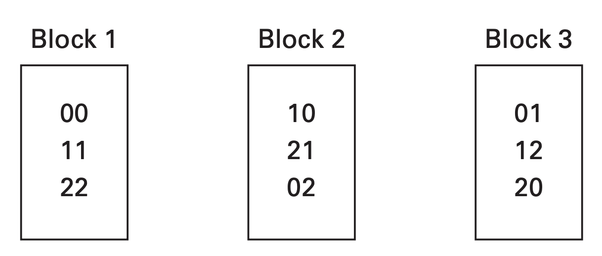
Note that the treatment combinations of principal block form a group with respect to addition (mod 3), i.e. addition of pair of treatment combination will lead to a treatment combination of the principal block. E.g.
$$\begin{array}{rlrlr}00+11=11& & 11+22=00& & 22+00=22\end{array}$$

---

Assignment of treatment combinations to blocks

Note that the treatment combinations in the other two blocks may be generated by adding (mod 3) any element of the new block to the elements of principal block. E.g.
$$\begin{array}{rlrlrl}\text{Block 2}& :00+02=02& & 11+02=10& & 22+02=21\\ \text{Block 3}& :00+20=20& & 11+20=01& & 22+20=12\end{array}$$

Example 9.2

The statistical analysis of the $3^2$ design confounded in three blocks is illustrated by using the following data

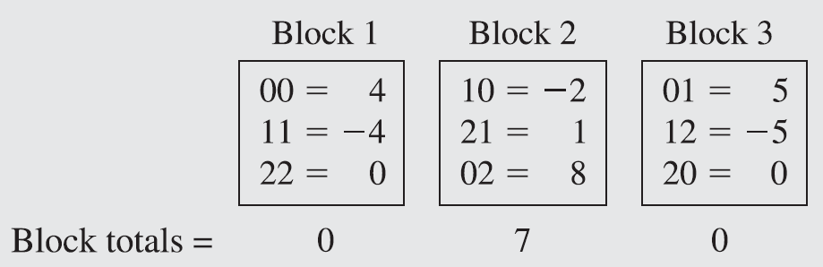
We find that

---

SS for main effects and interaction: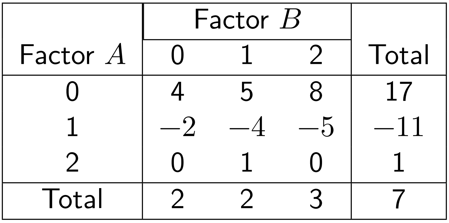

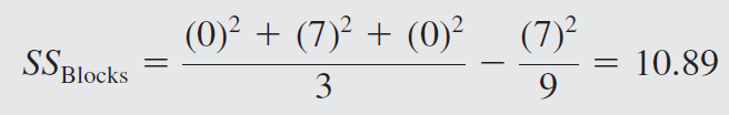
$$\begin{array}{c}S{S}_A:\frac{{17}^2+{11}^2+1^2}{3}-\frac{7^2}{9}=131.56\\ S{S}_B:\frac{2^2+2^2+3^2}{3}-\frac{7^2}{9}=0.22\\ S{S}_{AB}:\frac{4^2+3^2+0^2}{3}-\frac{7^2}{9}=2.89\\ S{S}_{A{B}^2}:\frac{0^2+0^2+7^2}{3}-\frac{7^2}{9}=10.89\end{array}$$

---

The I or ${AB}^2$ component of the $AB$ interaction may be found by computing the sum of squares between the left-to-right diagonal totals in the above layout. ${SS}_{\text{Blocks }}$ is exactly equal to the ${AB}^2$ component of interaction.

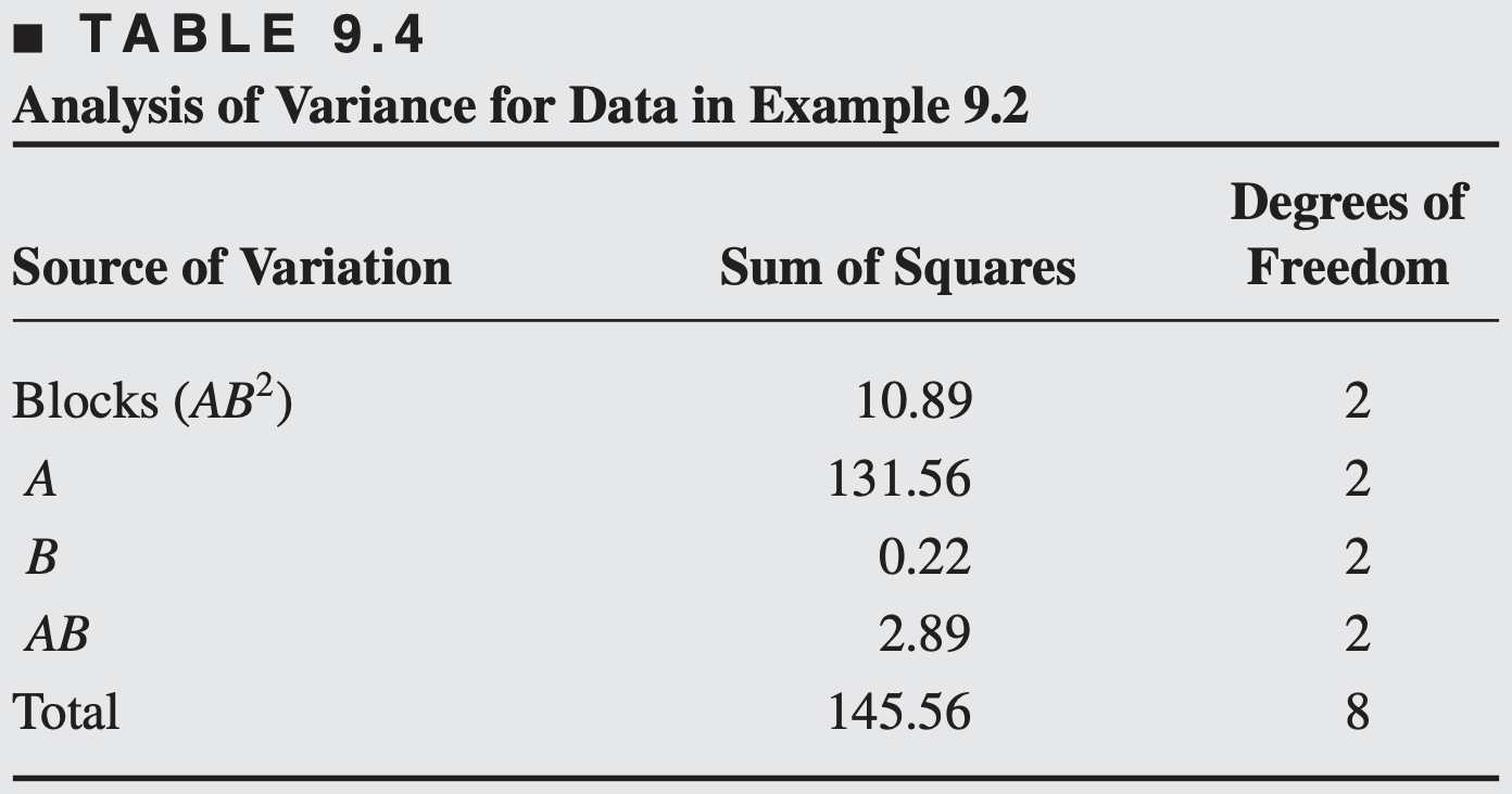
The analysis of variance is shown below. Because there is only one replicate, no formal tests can be performed. It is not a good idea to use the AB component of interaction as an estimate of error.

---

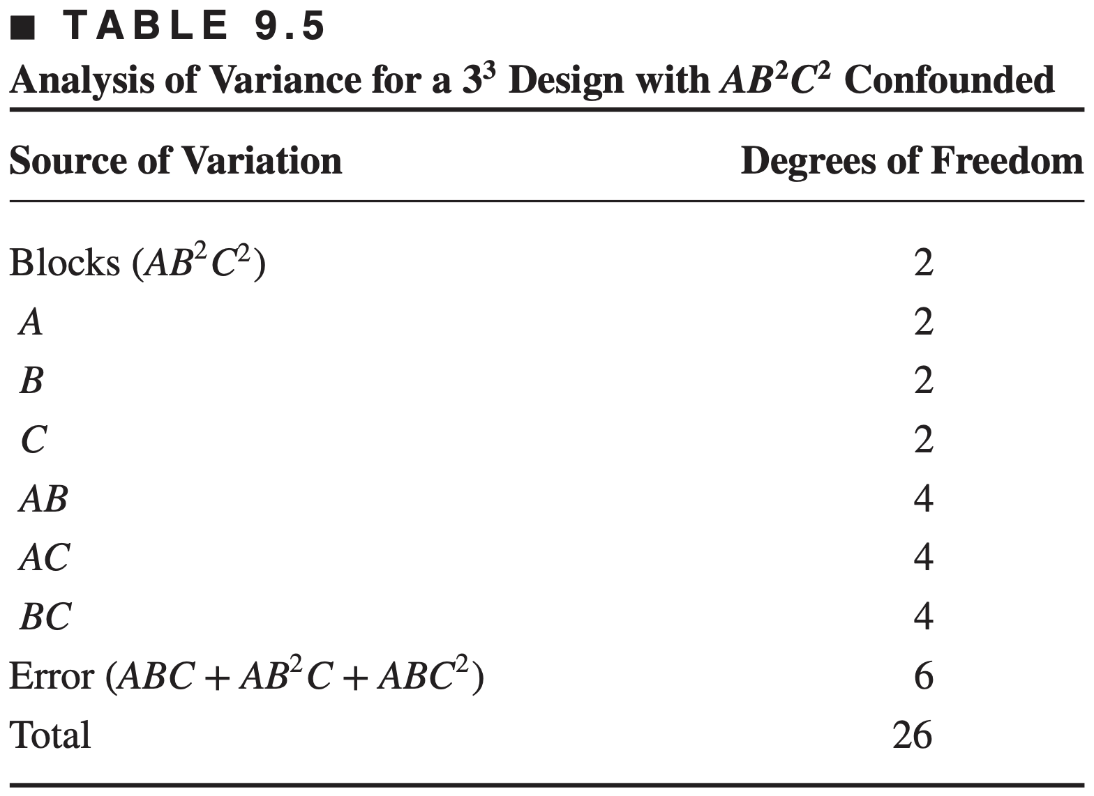
Slightly complicated example: The $3^3$ design confounded in three blocks of nine runs each. Suppose the $A{B}^2{C}^2$ component of the three-factor interaction will be confounded with blocks, the defining contrast is $$\begin{array}{rl}L& =x_1+2x_2+2x_3\end{array}$$ It is clear that the treatment combinations $000$, $110$ and $101$ are elements of principal block, other six elements of principal block can be obtained from these elements: $$\begin{array}{rlrlr}110+110=220& & 101+101=202& & 110+101=211\\ 220+101=021& & 202+220=122& & 202+110=012\end{array}$$

---

Treatment combinations of the principal block of the $3^3$ design with $A{B}^2{C}^2$ component confounded in three blocks.

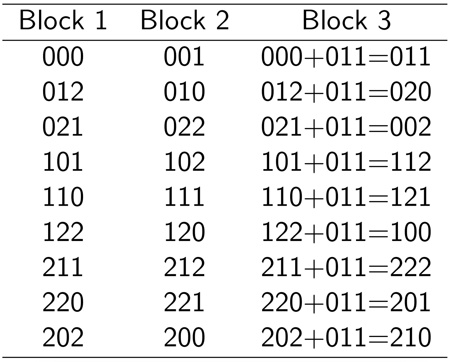
Treatment combinations of other two blocks can easily be obtained by adding a treatment combination (which is not in the principal block) to each element of the principal block

---

The $3^k$ factorial design in nine blocks

• If $3^k$ design is confounded in 9 blocks then 8 degrees of freedom is confounded with blocks.
• We need to choose two interaction components (4 degrees of freedom), which will result two more components will be confounded (4 degrees of freedom)
• E.g. if $P$ and $Q$ are two components that are selected for confounding then $PQ$ and $P{Q}^2$ will also be confounded with blocks
• There will be two defining contrasts $$\begin{array}{rl}{L}_1& ={\alpha }_1{x}_1+{\alpha }_2{x}_2+\cdots +{\alpha }_k{x}_k\\ L_2& ={\beta }_1{x}_1+{\beta }_2{x}_2+\cdots +{\beta }_k{x}_k\end{array}$$ 9 blocks can be constructed based on the values of $L_1$ and $L_2$ or using group-theoretic property of the principal block

---

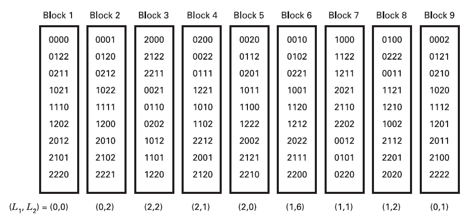
Consider the $3^4$ factorial design confounded in nine blocks of nine runs each.

Suppose we choose to confound $ABC$ and ${AB}^2{D}^2$. Their generalized interactions $$\begin{array}{rl}& (ABC)\left(A{B}^2{D}^2\right)=A^2{B}^{3}C{D}^2={\left(A^2{B}^{3}C{D}^2\right)}^2=A{C}^{2}D\\ & (ABC){\left(A{B}^2{D}^2\right)}^2=A^3{B}^{5}C{D}^4=B^{2}CD={\left(B^{2}CD\right)}^2={BC}^2{D}^2\end{array}$$ are also confounded with blocks. The defining contrasts for $ABC$ and ${AB}^2{D}^2$ are $$\begin{array}{c}{L}_1=x_1+x_2+x_3\\ L_2=x_1+2x_2+2x_4\end{array}$$

---

9.3 Fractions of $3^k$ factorial design

The one-third fraction of the $3^k$ factorial design

• The largest fraction of the $3^k$ design is a one-third fraction contains $3^{k-1}$ runs, which is known as $3^{k-1}$ fractional design

• To construct a $3^{k-1}$ fractional factorial design, select an interaction component (which has 2 degrees of freedom) and partition the full $3^k$ runs into three blocks.

• Each of the three resulting blocks is a $3^{k-1}$ fractional design, and any one of the blocks may be selected for use

• If $A{B}^{{\alpha }_2}{C}^{{\alpha }_3}\cdots K^{{\alpha }_k}$ is the component of interaction used to define the blocks, then the defining relation is $$\begin{array}{r}I=A{B}^{{\alpha }_2}{C}^{{\alpha }_3}\cdots K^{{\alpha }_k}\end{array}$$

• The alias structure for an effect can be obtained by multiplying the effect by both $I$ and $I^2$, e.g. alias structure of the main effect $A$ are $AI$ and $A{I}^2$.

---

• Example: To construct a one-third fraction of the $3^3$ design, we may consider any of the interaction components as defining relation.
• Since there are four interaction components, which are $ABC$, $AB{C}^2$, $A{B}^{2}C$, $A{B}^2{C}^2$, there will be 12 possible one-third fraction of the $3^3$ design and the defining contrast to obtain the designs $$\begin{array}{r}{x}_1+{\alpha }_2{x}_2+{\alpha }_3{x}_3=u(\text{mod}3)\end{array}$$ where $\alpha =1,2$ and $u=0,1,\text{or}2$.
• If we select the component $A{B}^2{C}^2$, the $3^{3-1}$ design will contain exactly 9 treatment combinations that must satisfy $$\begin{array}{r}{x}_1+2x_2+2x_3=u,(\text{mod}3)\end{array}$$ where $u=0,1,\text{or}2$.

---

The alias structure with the defining relation $I=A{B}^2{C}^2$: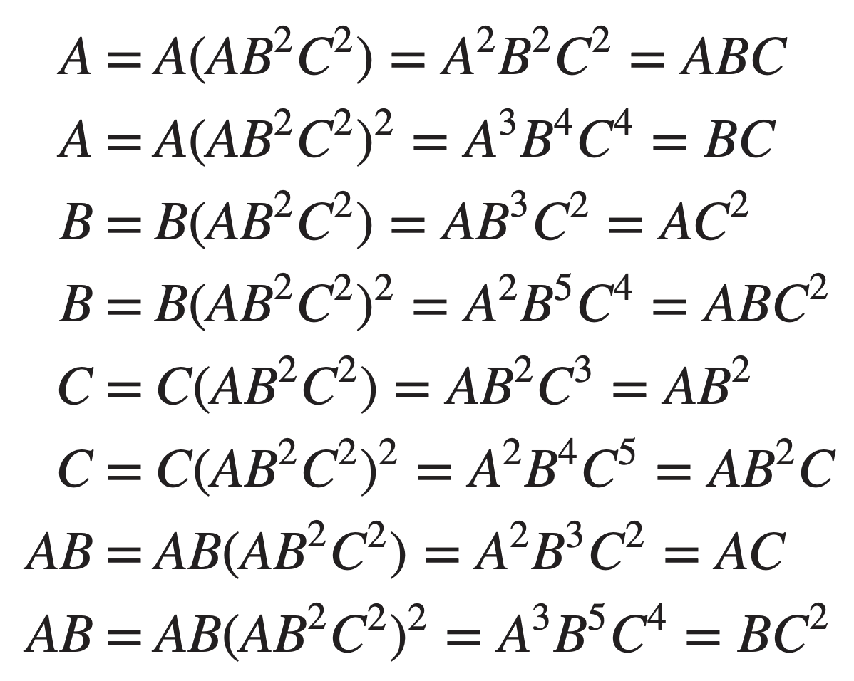

The four effects that are actually estimated from the eight degrees of freedom are: $A+BC+ABC$, $B+B{C}^2+AB{C}^2$, $C+A{B}^2+A{B}^{2}C$, $AB+AC+B{C}^2$

---

The treatment combinations in a $3^{k-1}$ design with the defining relation $$I=A{B}^{{\alpha }_2}{C}^{{\alpha }_3}\cdots K^{{\alpha }_k}$$ can be constructed as:

• Write down the $3^{k-1}$ runs for a full factorial design with $k-1$ factors, with the usual 0, 1, 2 notation.
• The $k^{\text{th}}$ factor is introduced by equating its levels $x_k$ to the appropriate component of the highest order interaction $A{B}^{{\alpha }_2}\cdots (K-1{)}^{{\alpha }_{k-1}}$ through the relationship $$\begin{array}{rl}{x}_k& ={\beta }_1{x}_1+\cdots +{\beta }_{k-1}{x}_{k-1},\end{array}$$ where ${\beta }_i=(3-{\alpha }_k){\alpha }_i$ (mod 3) for $1\le i\le k-1$. This yields a design of the highest possible resolution

---

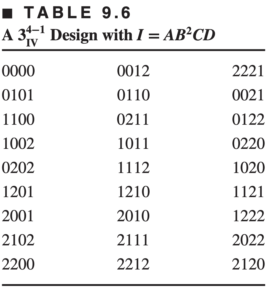
Consider a one-third fraction of the $3^4$ factorial design with $I=A{B}^{2}CD$, i.e. $x_1+2x_2+x_3+x_4=u(\text{mod}3)$.

First construct the $3^3$ design in factor $A$, $B$, and $C$: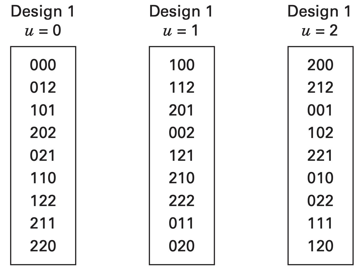

Levels for the factor $D$ can be obtained from $$x_4={\beta }_1{x}_1+{\beta }_2{x}_2+{\beta }_3{x}_3,{\beta }_i=(3-{\alpha }_4){\alpha }_i,i=1,2,3$$

---

Defining relation: $x_1+2x_2+x_3+x_4=u(\text{mod}3)$ $\Rightarrow {\alpha }_1=1,{\alpha }_2=2,{\alpha }_3=1,{\alpha }_4=1$ Levels for factor D: $x_4={\beta }_1{x}_1+{\beta }_2{x}_2+{\beta }_3{x}_3$, where ${\beta }_1=(3-{\alpha }_4){\alpha }_1=2$, ${\beta }_2=1$, and ${\beta }_3=2$ $\Rightarrow x_4=2x_1+x_2+2x_3$

As an example, alias structure for the effect $A$ is $A(A{B}^{2}CD)=A^2{B}^{2}CD=AB{C}^2{D}^2$, $A(A{B}^{2}CD{)}^2=B{C}^2{D}^2$

Resolution??

The general $3^{k-p}$ fractional factorial design

• The $3^{k-p}$ fractional factorial design is th $(1/3{)}^p$ fraction of the $3^k$ design for $p<k$, where the fraction contains $3^{k-p}$ runs.
• The construction of $3^{k-p}$ includes the selection of $p$ components of interaction first, which is then used to partition $3^k$ treatment combinations into $3^p$ blocks. Each block is a $3^{k-p}$ fractional factorial design.
• The defining relation $I$ of any fraction consists of $p$ initially chosen components and their $(3^p-2p-1)/2$ generalized interactions.
  
• Alias structure of an effect can be obtained by multiplying the effect by the defining relation $I$ and $I^2$
• The $3^{k-p}$ fractional factorial design can also be obtained by writing down the full $3^{k-p}$ design first in $(k-p)$ factors and then levels of additional $p$ factors are obtained from the corresponding defining contrasts.