| Temperature (\(\xi_1\)) | Pressure Ratio (\(\xi_2\)) | Purity |
|---|---|---|
| -225 | 1.1 | 82.8 |
| -225 | 1.3 | 83.5 |
| -215 | 1.1 | 84.7 |
| -215 | 1.3 | 85.0 |
| -220 | 1.2 | 84.1 |
| -220 | 1.2 | 84.5 |
| -220 | 1.2 | 83.9 |
| -220 | 1.2 | 84.3 |
Chapter 11
(AST301) Design and Analysis of Experiments II
11 Response Surface Methods and Designs
11.1 Introduction
Factorial designs are very useful for factor screening - that is, identifying the most important factors that affect the performance of a process. Sometimes this is called process characterization.
Once the appropriate subset of process variables is identified, the next step is usually process optimization, or finding the set of operating conditions for the process variables that result in the best process performance.
Response surface methodology, or RSM, is a collection of mathematical and statistical techniques useful for the modeling and analysis of problems in which a response of interest is influenced by several variables and the objective is to optimize this response.
For example, suppose that a chemical engineer wishes to find the levels of temperature \(\left(x_1\right)\) and pressure \(\left({x}_2\right)\) that maximize the yield \(({y})\) of a process.
The process yield is a function of the levels of temperature and pressure, say \[ y=f\left(x_1, x_2\right)+\epsilon \] where \(\epsilon\) represents the noise or error observed in the response \(y\). If we denote the expected response by \[ E(y)=f\left(x_1, x_2\right)=\eta \] then the surface represented by \[ \eta=f\left(x_1, x_2\right) \] is called a response surface.
We usually represent the response surface graphically, where \(\eta\) is plotted versus the levels of \(x_1\) and \(x_2\)
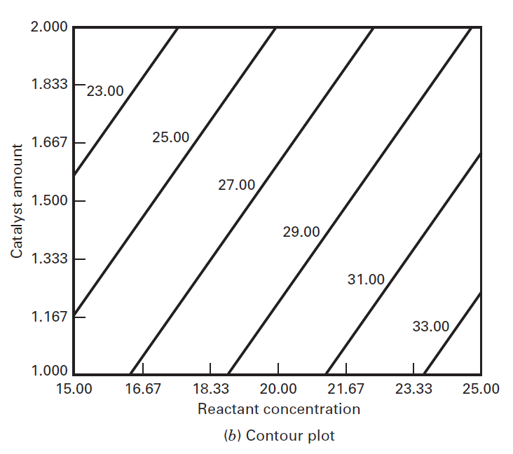
To help visualize the shape of a response surface, we often plot the contours of the response surface.
In the contour plot, lines of constant response are drawn in the \(x_1, x_2\) plane. Each contour corresponds to a particular height of the response surface.
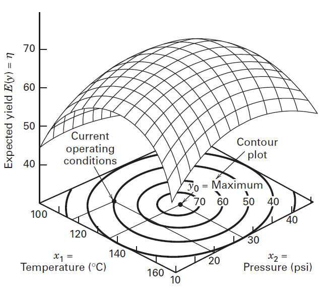
Figure: A three-dimensional response surface showing the expected yield of temperature \(\left({x}_1\right)\) and pressure \(\left({x}_2\right)\) with a contour plot.
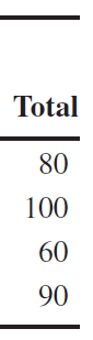
As an example, consider an investigation into the effect of the concentration of the reactant and the amount of the catalyst on the conversion (yield) in a chemical process.
The objective of the experiment is to determine if adjustments to either of these two factors would increase the yield.
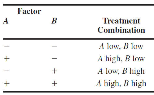
Let the reactant concentration be factor \(A\) and let the two levels of interest be 15 and 25 percent. The catalyst is factor \(B\) and let the two levels of interest be 2 pounds and 1 pound.
The experiment is replicated three times, so there are 12 runs. The order in which the runs are made is random, so this is a completely randomized experiment.
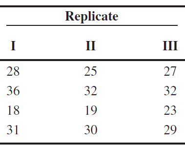
On the basis of the \(p-\)values, we conclude that the main effects are statistically significant and that there is no interaction between these factors.
The Response Surface
The regression model \[ \hat{y}=27.5+\left(\frac{8.33}{2}\right) x_1+\left(\frac{-5.00}{2}\right) x_2 \] can be used to generate response surface plots. If it is desirable to construct these plots in terms of the natural factor levels, then we simply substitute the relationships between the natural and coded variables that we gave earlier into the regression model, yielding
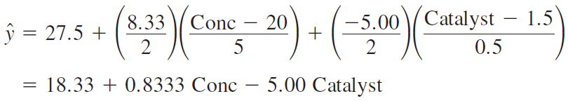
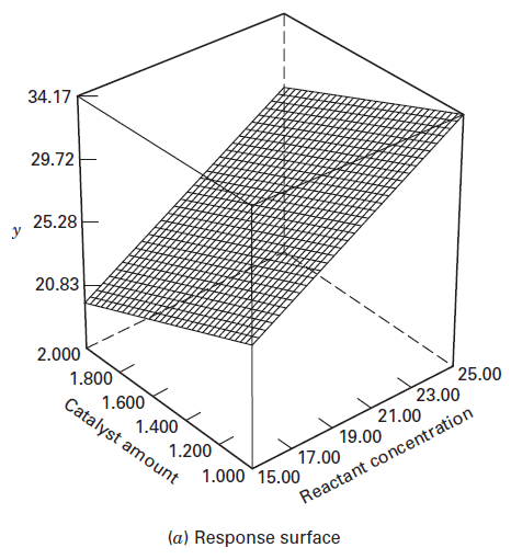
Because the model is first-order (that is, it contains only the main effects), the fitted response surface is a plane.
From examining the contour plot, we see that yield increases as reactant concentration increases and catalyst amount decreases.
Often, we use a fitted surface such as this to find a direction of potential improvement for a process.
RSM
In most RSM problems, the form of the relationship between the response and the independent variables is unknown.
Thus, the first step in RSM is to find a suitable approximation for the true functional relationship between \(y\) and the set of independent variables.
Usually, a low-order polynomial in some region of the independent variables is employed.
If the response is well modeled by a linear function of the independent variables, then the approximating function is the first-order model \[ y=\beta_0+\beta_1 x_1+\beta_2 x_2+\cdots+\beta_k x_k+\epsilon \]
If there is curvature in the system, then a polynomial of higher degree must be used, such as the second-order model \[ y=\beta_0+\sum_{i=1}^k \beta_i x_i+\sum_{i=1}^k \beta_{i i} x_i^2+\sum_{i<j} \beta_{i j} x_i x_j+\epsilon. \]
Almost all RSM problems use one or both of these models.
The method of least squares is used to estimate the parameters in the approximating polynomials.
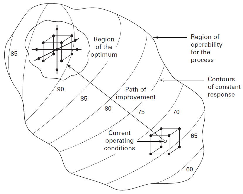
RSM is a sequential procedure.
Often, when we are at a point on the response surface that is remote from the optimum, the objective is to lead the experimenter rapidly and efficiently along a path of improvement toward the general vicinity of the optimum.
Once the region of the optimum has been found, a more elaborate model, such as the second-order model, may be employed, and an analysis may be performed to locate the optimum.
Summary: (Steps of RSM)
- Find a suitable approximation for \(y=f(\mathbf{x})\) using LS {maybe a low-order polynomial}
- Move towards the region of the optimum
- When curvature is found find a new approximation for \(y=f(\mathbf{x})\) {generally a higher order polynomial} and perform the “Response Surface Analysis”
The eventual objective of RSM is to determine the optimum operating conditions for the system or to determine a region of the factor space in which operating requirements are satisfied.
11.2 Method of Steepest Ascent
(A procedure for moving sequentially from an initial “guess” towards to region of the optimum)
Frequently, the initial estimate of the optimum operating conditions for the system will be far from the actual optimum.
In such circumstances, the objective of the experimenter is to move rapidly to the general vicinity of the optimum.
When we are remote from the optimum, we usually assume that a first-order model is an adequate approximation to the true surface in a small region of the \(x\)’s.
The method of steepest ascent is a procedure for moving sequentially in the direction of the maximum increase in the response.
If minimization is desired, then we call this technique the method of steepest descent.
The fitted first-order model is \[ \hat{y}=\hat{\beta}_0+\sum_{i=1}^k \hat{\beta}_i x_i \] and the first-order response surface, that is, the contours of \(\hat{y}\), is a series of parallel lines.
The direction of steepest ascent is the direction in which \(\hat{y}\) increases most rapidly.
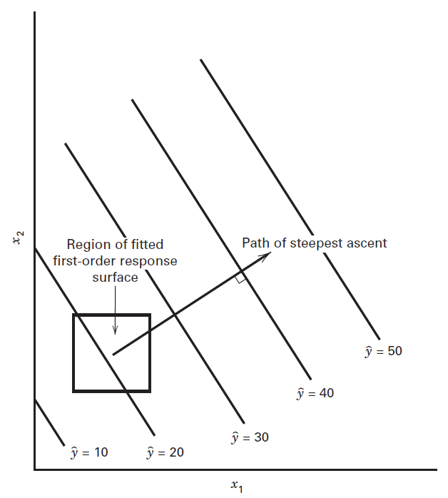
We usually take as the path of steepest ascent the line through the center of the region of interest and normal to the fitted surface.
Thus, the steps along the path are proportional to the regression coefficients.
The actual step size is determined by the experimenter based on process knowledge or other practical considerations.
Experiments are conducted along the path of steepest ascent until no further increase in response is observed.
Then a new first-order model may be fit, a new path of steepest ascent determined, and the procedure continued.
Eventually, the experimenter will arrive in the vicinity of the optimum. This is usually indicated by lack of fit of a first-order model. At that time, additional experiments are conducted to obtain a more precise estimate of the optimum.
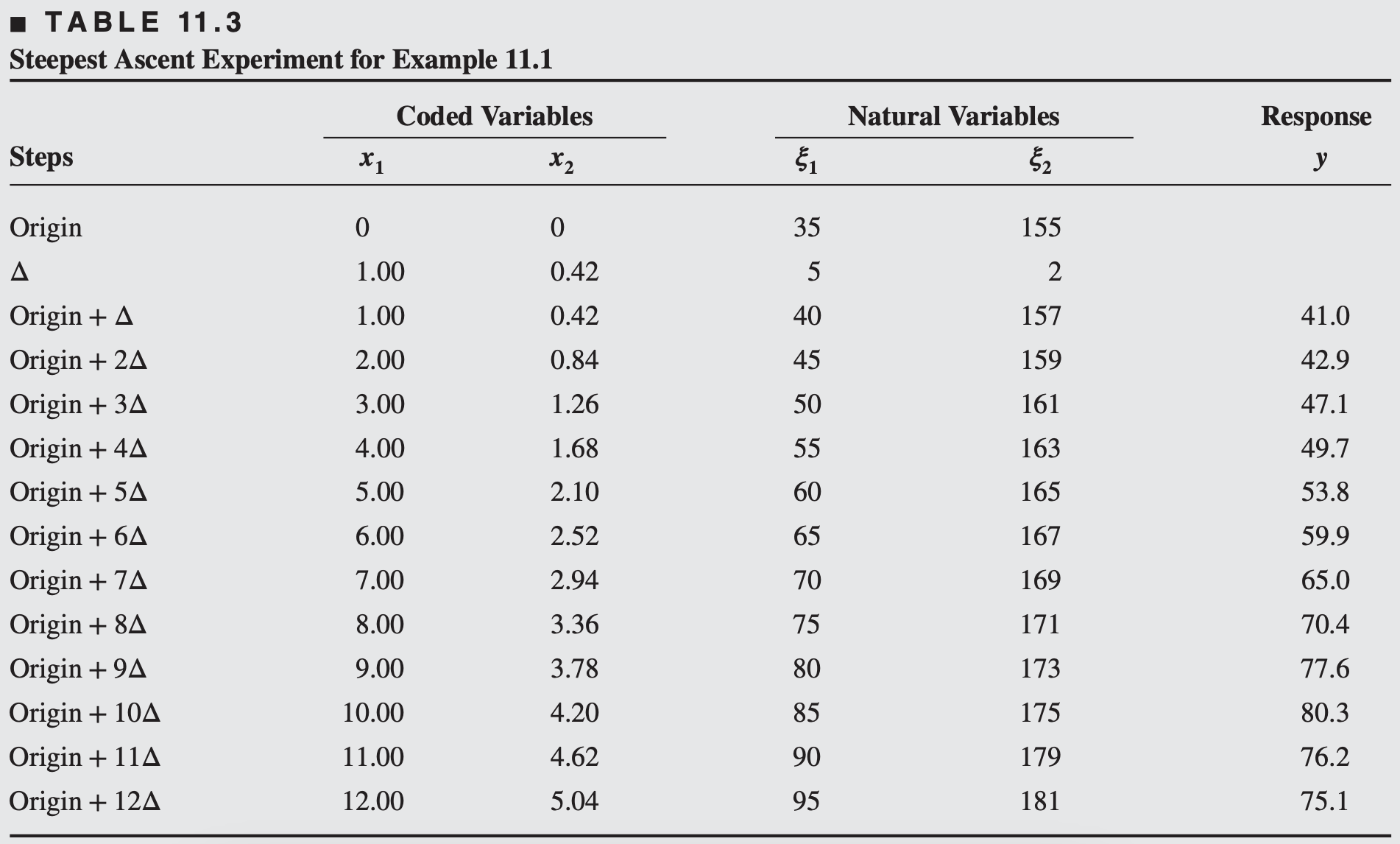
Example 11.1
A chemical engineer is interested in determining the operating conditions that maximize the yield of a process. Two controllable variables influence process yield: reaction time and reaction temperature. The engineer is currently operating the process with a reaction time of 35 minutes and a temperature of \(155^{\circ} \mathrm{F}\), which result in yields of around 40 percent. Because it is unlikely that this region contains the optimum, she fits a first-order model and applies the method of steepest ascent.
The engineer decides that the region of exploration for fitting the first-order model should be \((30,40)\) minutes of reaction time and \((150,160)\) Fahrenheit. To simplify the calculations, the independent variables will be coded to the usual \((-1,1)\) interval. Thus, if \(\xi_1\) denotes the natural variable time and \(\xi_2\) denotes the natural variable temperature, then the coded variables are \[ x_1=\frac{\xi_1-35}{5} \quad \text { and } \quad x_2=\frac{\xi_2-155}{5} \]
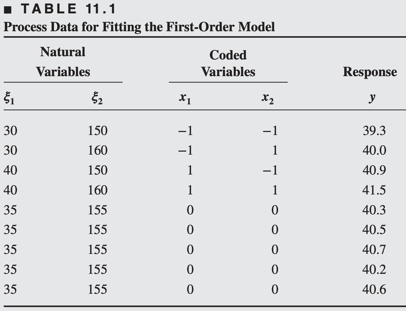
Note that the design used to collect these data is a \(2^2\) factorial augmented by five center points.
Replicates at the center are used to estimate the experimental error and to allow for checking the adequacy of the first-order model. Also, the design is centered about the current operating conditions for the process.
A first-order model may be fit to these data by least squares. Employing the methods for two-level designs, we obtain the following model in the coded variables \[ \hat{y}=40.44+0.775 x_1+0.325 x_2 \]
Before exploring along the path of steepest ascent, the adequacy of the first-order model should be investigated.
The \(2^2\) design with center points allows the experimenter to do the following:
- Obtain an estimate of error.
- Check for interactions (cross-product terms) in the model.
- Check for quadratic effects (curvature) (See Section 11.2.3 for details).
The replicates at the center can be used to calculate an estimate of error as follows: \[ \hat{\sigma}^2= \frac{(40.3)^2+(40.5)^2+(40.7)^2+(40.2)^2 +(40.6)^2-(202.3)^2 / 5}{4} =0.0430 \]
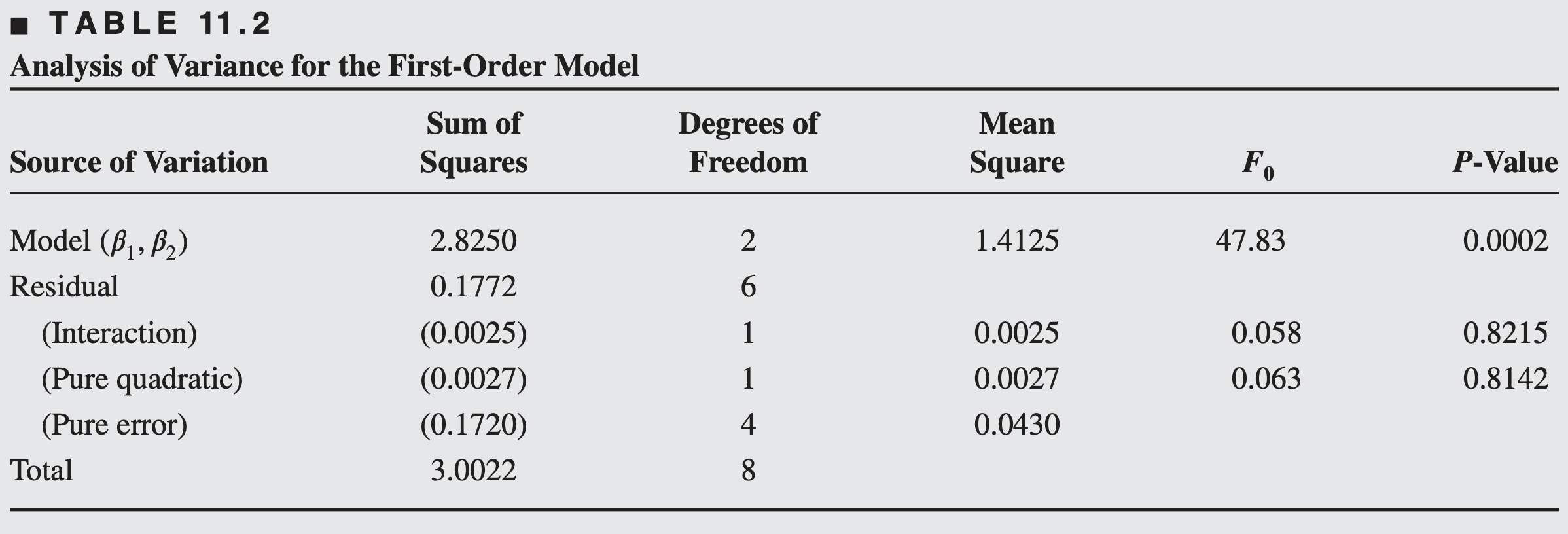
- we have no reason to question the adequacy of the first-order model
To move away from the design center-the point \((x_1=0,x_2=0)\) along the path of steepest ascent, we would move 0.775 units in the \(x_1\) direction for every 0.325 units in the \(x_2\) direction.
Thus, the path of steepest ascent passes through the point \(\left(x_1=0, x_2=0\right)\) and has a slope \(0.325 / 0.775\).
The engineer decides to use 5 minutes of reaction time as the basic step size. Using the relationship between \(\xi_1\) and \(x_1\), we see that 5 minutes of reaction time is equivalent to a step in the coded variable \(x_1\) of \(\Delta x_1=1\). Therefore, the steps along the path of steepest ascent are \(\Delta x_1=1.0000\) and \(\Delta x_2=(0.325 / 0.775)=0.42\).
- The engineer computes points along this path and observes the yields at these points until a decrease in response is noted
A new first-order model is fit around the point \((\xi_1=85, \xi_2=175)\). The region of exploration for \(\xi_1\) is [80, 90], and it is \([170,180]\) for \(\xi_2\). Thus, the coded variables are \[ x_1=\frac{\xi_1-85}{5} \quad \text { and } \quad x_2=\frac{\xi_2-175}{5} \]
Once again, a \(2^2\) design with five center points is used. The experimental design is shown in Table 11.4.
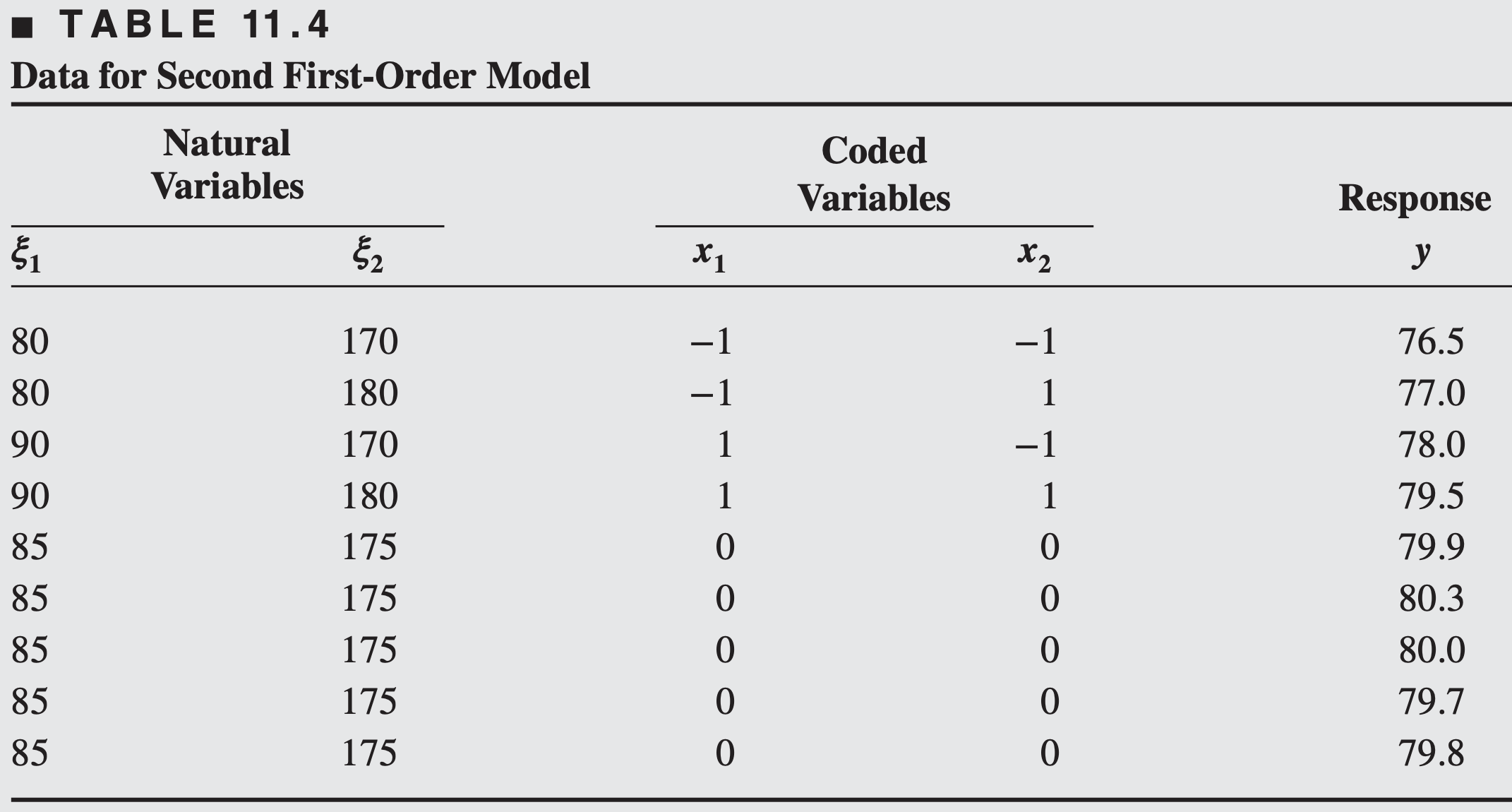
The first-order model fit to the coded variables in Table 11.4 is \[ \hat{y}=78.97+1.00 x_1+0.50 x_2 \]
The analysis of variance for this model, including the interaction and pure quadratic term checks, is shown in Table 11.5.
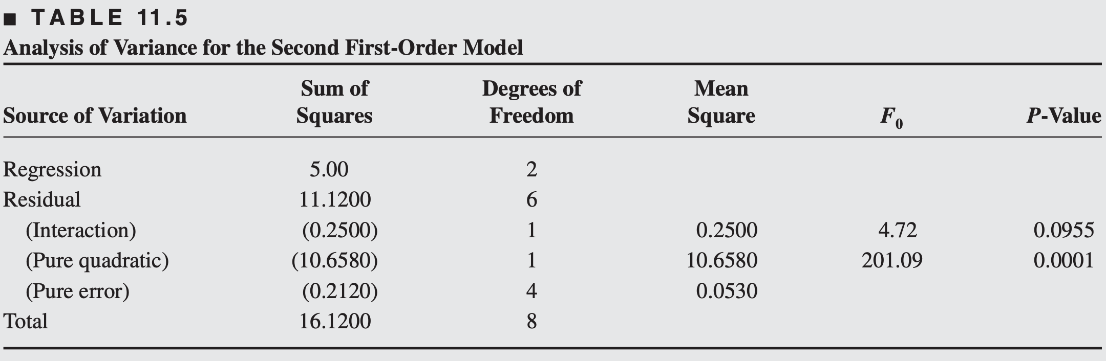
The interaction and pure quadratic checks imply that the first-order model is not an adequate approximation.
This curvature in the true surface may indicate that we are near the optimum.
At this point, additional analysis must be done to locate the optimum more precisely.
Step-by-step procedure
Choose a step size in one of the process variables, say \(\Delta x_j\). Usually, we would select the variable we know the most about, or we would select the variable that has the largest absolute regression coefficient \(\left|\hat{\beta}_j\right|\).
The step size in the other variables is \[ \Delta x_i=\frac{\hat{\beta}_i}{\hat{\beta}_j / \Delta x_j} \quad i=1,2, \ldots, k \quad i \neq j \]
Convert the \(\Delta x_i\) from coded variables to the natural variables.
Test for Curvature
By using two-level factorial and fractional factorial designs (augmented with center points), the experimenter is able to
- Obtain an estimate of pure error.
- The replicated center points can be used to calculate an estimate of the pure error \(\hat{\sigma}^2=s^2\) where \(s^2\) is the sample variance of the center point responses.
- Overall check for interaction effects in the model.
- The sum of squares for testing for interaction is found by accumulating sum of squares associated with all two-factor interaction terms which can be estimated.
- Overall check for quadratic effects (curvature).
If there is no curvature present, then the average response corresponding to the factorial points (say \(\bar{{y}}_{{F}}\)) should be similar to the average response corresponding to the center points (say \(\bar{{y}}_{{C}}\)).
Thus, \(\bar{{y}}_{{F}}-\bar{{y}}_{{C}}\) is an measure of the overall curvature in the surface over that design space.
If the difference \(\bar{{y}}_{{F}}-\bar{{y}}_{{C}}\) is small, then there is no quadratic curvature.
On the other hand, if \(\bar{{y}}_{{F}}-\bar{{y}}_{{C}}\) is large, then quadratic curvature is present. A single-degree-of-freedom sum of squares for pure quadratic curvature is given by \[ S S_{\text {Pure quadratic }}=\frac{n_F n_C\left(\bar{y}_F-\bar{y}_C\right)^2}{n_F+n_C} \] where, in general, \({n}_{{F}}\) is the number of factorial design points and \({n}_{{C}}\) is the number of centre point.
- When points are added to the center of the \(2^{{k}}\) design, the test for curvature actually tests the hypotheses \[ \begin{aligned} & H_0: \sum_{j=1}^k \beta_{j j}=0 \\ & H_1: \sum_{j=1}^k \beta_{j j} \neq 0 \end{aligned} \]
Further reading: https://online.stat.psu.edu/stat503/lesson/11
Exercises
11.1. A chemical plant produces oxygen by liquefying air and separating it into its component gases by fractional distillation. The purity of the oxygen is a function of the main condenser temperature and the pressure ratio between the upper and lower columns. Current operating conditions are temperature \(\left(\xi_1\right)=-200^{\circ} \mathrm{C}\) and pressure ratio \(\left(\xi_2\right)=1.2\). Using the following data, find the path of steepest ascent:
11.4. For the first-order model \[ \hat{y}=60+1.5 x_1-0.8 x_2+2.0 x_3 \] find the path of steepest ascent. The variables are coded as \(-1 \leq x_i \leq 1\)
11.5. The region of experimentation for three factors are time ( \(40 \leq T_1 \leq 80 \mathrm{~min}\) ), temperature \(\left(200 \leq T_2 \leq 300^{\circ} \mathrm{C}\right)\), and pressure ( \(20 \leq P \leq 50 \mathrm{psig}\) ). A first-order model in coded variables has been fit to yield data from a \(2^3\) design. The model is \[ \hat{y}=30+5 x_1+2.5 x_2+3.5 x_3 \]
Is the point \(T_1=85, T_2=325, P=60\) on the path of steepest ascent?