Chapter 6

(AST301) Design and Analysis of Experiments II

6 The $2^k$ Factorial Design

6.1 Introduction

• Factorial designs are widely used in experiments involving several factors where it is necessary to study the joint effect of the factors on a response.

• Chapter 5 presented general methods for the analysis of factorial designs.

• However, several special cases of the general factorial design are important because they are widely used in research work and also because they form the basis of other designs of considerable practical value.

---

• The most important of these special cases is that of $k$ factors, each at only two levels.

• These levels may be quantitative, such as two values of temperature, pressure, or time; or they may be qualitative, such as two machines, two operators, the “high” and “low” levels of a factor, or perhaps the presence and absence of a factor.

• A complete replicate of such a design requires $2\times 2\times \cdots \times 2=2^k$ observations and is called a $2^k$ factorial design.

• This chapter focuses on this extremely important class of designs. Throughout this chapter, we assume that

  1. the factors are fixed,
  2. the designs are completely randomized, and
  3. the usual normality assumptions are satisfied.

---

The $2^k$ design is particularly useful in the early stages of experimental work when many factors are likely to be investigated.

It provides the smallest number of runs with which $k$ factors can be studied in a complete factorial design.

Consequently, these designs are widely used in factor screening experiments (where the experiments is intended in discovering the set of active factors from a large group of factors).

6.2 The $2^2$ design

• The first design in the $2^k$ series is one with only two factors, say $A$ and $B$, each run at two levels.

• This design is called a $2^2$ factorial design.

• The levels of the factors may be arbitrarily called “low” and “high.”

---

• Consider an investigation into the effect of the concentration of the reactant (factor A) and the amount of catalyst (factor B) on the yield in a chemical process.

  • Levels of factor A: 15 and 25 percent
  • Levels of factor B: 1 and 2 pounds

• The objective of the experiment is to determine if adjustments to either of these two factors would increase the yield.

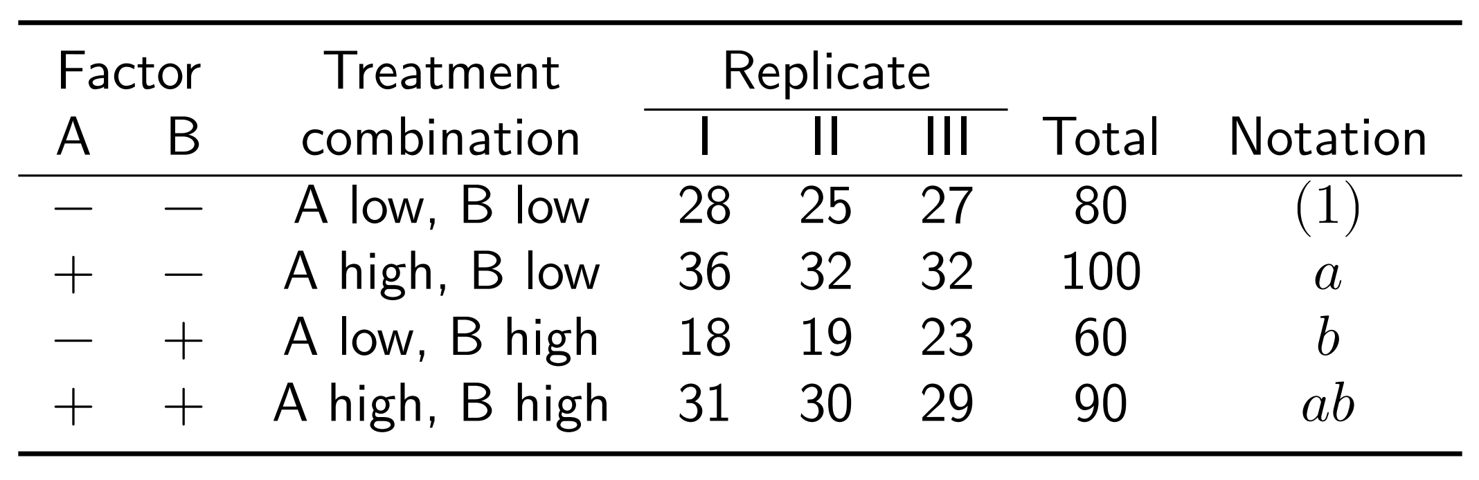
• The experiment is replicated three times, so there are 12 runs. The order in which the runs are made is random, so this is a completely randomized experiment.

---

Data layout:

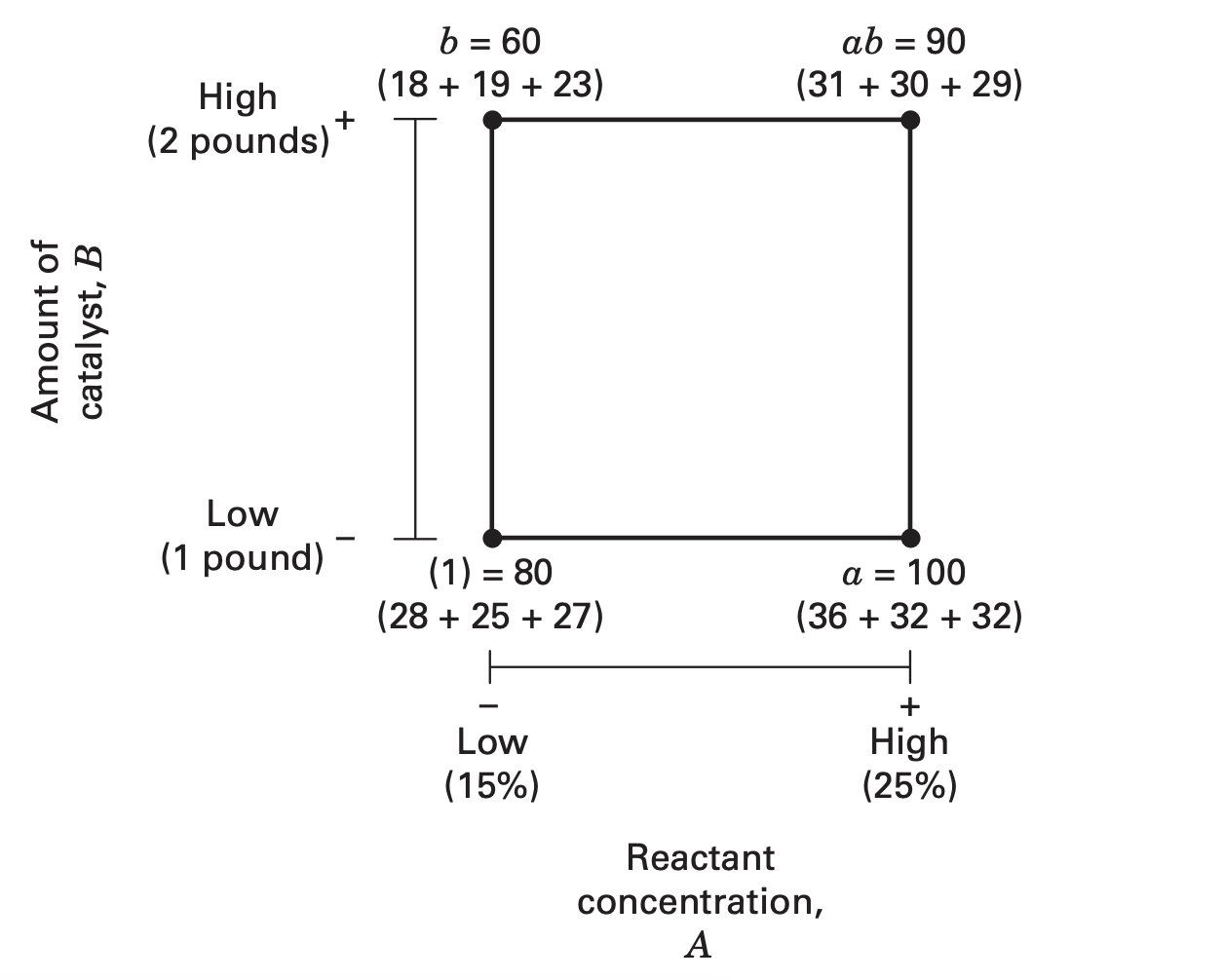
Graphical view:

---

By convention, we denote the effect of a factor by a capital Latin letter.

• “A” refers to the effect of factor A,

• “B” refers to the effect of factor B, and

• “AB” refers to the AB interaction.

• The four treatment combinations in the design are represented by lowercase letters.

---

• The high level of any factor in the treatment combination is denoted by the corresponding lowercase letter and that the low level of a factor in the treatment combination is denoted by the absence of the corresponding letter.

• Thus $a$ represents the treatment combination of $A$ at the high level and $B$ at the low level, $b$ represents $A$ at the low level and $B$ at the high level, and $ab$ represents both factors at the high level.

• By convention, (1) is used to denote both factors at the low level.

• This notation is used throughout the $2^k$ series.

---

• In a two-level factorial design the average effect of a factor is defined as the change in response produced by a change in the level of that factor averaged over the levels of the other factor.

• The symbols (1), $a$, $b$, and $ab$ represent the total of the response observation at all $n$ replicates taken at the treatment combination.

• The effect of $A$ at the low level of B is $[a-(1)]/n$, and the effect of $A$ at the high level of $B$ is $[ab-b]/n$. Averaging these two quantities yields the main effect of $A$: $$\begin{array}{rl}A& =\frac{1}{2}\{\frac{[ab-b]+[a-(1)]}{n}\}\\ & =\frac{1}{2n}[ab+a-b-(1)]\end{array}$$

---

• The main effect of $B$ is: $$\begin{array}{rl}B& =\frac{1}{2}\{\frac{[ab-a]+[b-(1)]}{n}\}\\ & =\frac{1}{2n}[ab+b-a-(1)]\end{array}$$

• We define the interaction effect $AB$ as the average difference between the effect of $A$ at the high level of $B$ and the effect of $A$ at the low level of $B$. Thus, $$\begin{array}{rl}AB& =\frac{1}{2}\{\frac{[ab-b]-[a-(1)]}{n}\}\\ & =\frac{1}{2n}[ab+(1)-a-b](6.3)\end{array}$$

• Alternatively, we may define $AB$ as the average difference between the effect of $B$ at the high level of A and the effect of $B$ at the low level of A. This will also lead to Equation 6.3.

---

$$\begin{array}{rl}A& =\frac{1}{2(3)}(90+100-60-80)=8.33\\ B& =\frac{1}{2(3)}(90+60-100-80)=-5.00\\ AB& =\frac{1}{2(3)}(90+80-100-60)=1.67\end{array}$$

---

• The effect of A (reactant concentration) is positive; this suggests that increasing A from the low level $(15\mathrm{\%})$ to the high level $(25\mathrm{\%})$ will increase the yield.

• The effect of B (catalyst) is negative; this suggests that increasing the amount of catalyst added to the process will decrease the yield.

• The interaction effect appears to be small relative to the two main effects.

The magnitude and direction of factor effects can be used to determine the important factor and ANOVA can generally be used to confirm the interpretation.*

Sum of squares

• Now we consider determining the sums of squares for $A$, $B$, and $AB$.

• Note that, in estimating A, a contrast is used: $$\begin{array}{r}A=\frac{1}{2n}[ab+a-b-(1)]=(\frac{1}{2n}){\text{Contrast}}_A\end{array}$$ Similarly, $$\begin{array}{rl}B& =\frac{1}{2n}[ab-a+b-(1)]=(\frac{1}{2n}){\text{Contrast}}_B\\ \\ AB& =\frac{1}{2n}[ab-a-b+(1)]=(\frac{1}{2n}){\text{Contrast}}_{AB}\end{array}$$

• The three contrasts — ${\text{Contrast}}_A$, ${\text{Contrast}}_B$, and ${\text{Contrast}}_{AB}$ — are orthogonal.

---

The sum of squares for any contrast is equal to the contrast squared divided by the number of observations in each total in the contrast times the sum of the squares of the contrast coefficients. $$S{S}_A=(\frac{1}{2^{2}n}){\text{Contrast}}_A^2=\frac{1}{4n}[ab+a-b-(1){]}^2$$

---

$$\begin{array}{rl}S{S}_A& =(\frac{1}{2^{2}n}){\text{Contrast}}_A^2=\frac{1}{4n}[ab+a-b-(1){]}^2\\ \\ S{S}_B& =(\frac{1}{2^{2}n}){\text{Contrast}}_B^2=\frac{1}{4n}[ab-a+b-(1){]}^2\\ \\ S{S}_{AB}& =(\frac{1}{2^{2}n}){\text{Contrast}}_{AB}^2=\frac{1}{4n}[ab-a-b+(1){]}^2\end{array}$$ Total sum of squares $$\begin{array}{rl}S{S}_T& =\sum _i\sum _j\sum _k{y}_{ijk}^2-\frac{y_{\cdot \cdot \cdot }^2}{4n}\end{array}$$ Error sum of square $$\begin{array}{rl}S{S}_E& =S{S}_T-S{S}_A-S{S}_B-S{S}_{AB}\end{array}$$

---

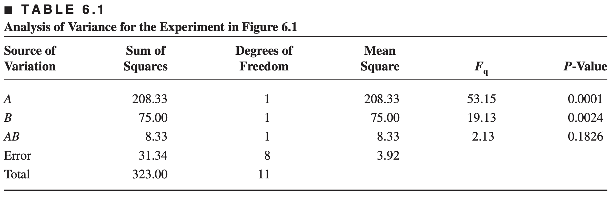
$$\begin{array}{rl}S{S}_A& =(\frac{1}{2^{2}n}){\text{Contrast}}_A^2=\frac{1}{4n}[ab+a-b-(1){]}^2=208.333\\ \\ S{S}_B& =(\frac{1}{2^{2}n}){\text{Contrast}}_B^2=\frac{1}{4n}[ab-a+b-(1){]}^2=75\\ \\ S{S}_{AB}& =(\frac{1}{2^{2}n}){\text{Contrast}}_{AB}^2=\frac{1}{4n}[ab-a-b+(1){]}^2=8.333\end{array}$$ Total sum of squares $$\begin{array}{rl}S{S}_T& =\sum _i\sum _j\sum _k{y}_{ijk}^2-\frac{y_{\cdot \cdot \cdot }^2}{4n}=323\end{array}$$ Error sum of square $$\begin{array}{rl}S{S}_E& =S{S}_T-S{S}_A-S{S}_B-S{S}_{AB}=31.333\end{array}$$

Analysis of Variance table

• On the basis of the p-values, we conclude that the main effects are statistically significant and that there is no interaction between these factors. This confirms our initial interpretation of the data based on the magnitudes of the factor effects.

Standard order of treatment combinations

• Treatment combinations written in the order $(1),a,b,ab$ is known as standard order or Yates’ order.

• Using this standard order, we see that the contrast coefficients used in estimating the effects are

• Note that the contrast coefficients for estimating the interaction effect are just the product of the corresponding coefficients for the two main effects.

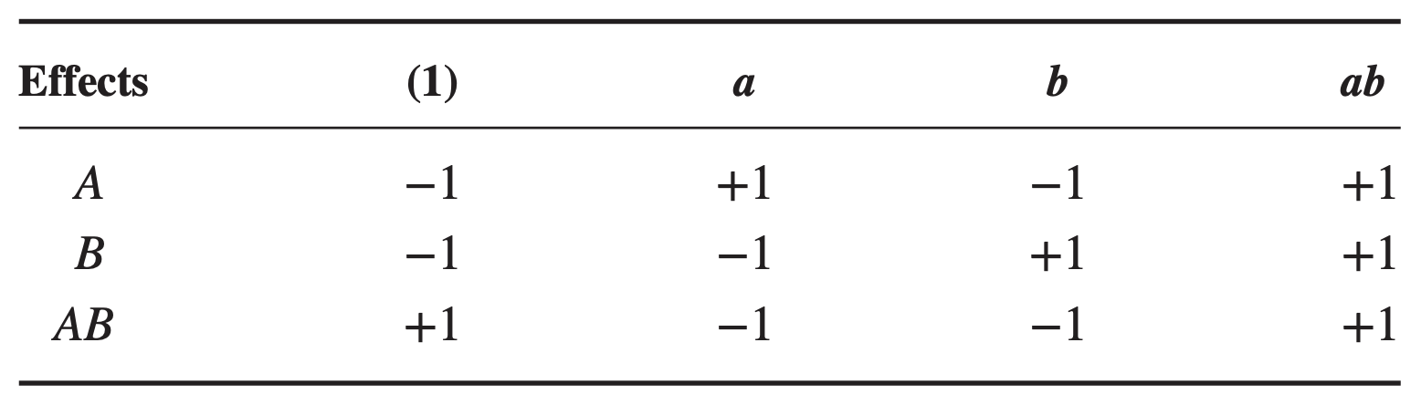
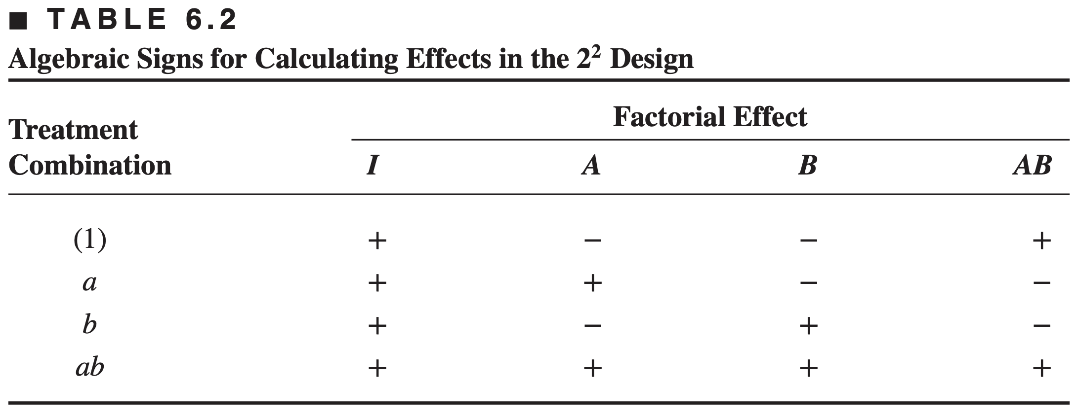
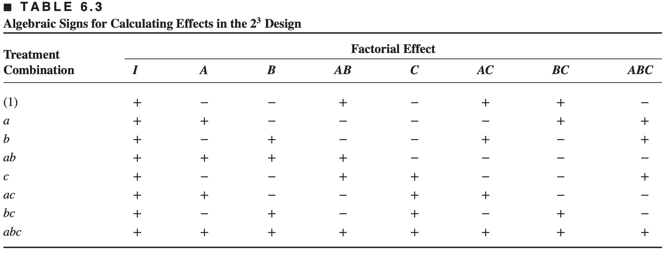
Algebraic signs for calculating effects in $2^2$ design

• The contrast coefficient is always either +1 or −1, and a table of plus and minus signs such as in Table 6.2 can be used to determine the proper sign for each treatment combination

• The symbol “I” indicates the total or average of the entire experiment.

• To find the contrast for estimating any effect, simply multiply the signs in the appropriate column of the table by the corresponding treatment combination and add.

  • For example, to estimate $A$, the contrast is $-(1)+a-b+ab.$

---

• The contrasts for the effects $A,B$, and $AB$ are orthogonal. Thus, the $2^2$ (and all $2^{\mathrm{k}}$ designs) is an orthogonal design.

• The $\pm 1$ coding for the low and high levels of the factors is often called the orthogonal coding or the effects coding.

Regression model

• In a $2^k$ factorial design, it is easy to express the results of the experiment in terms of a regression model.

• For the chemical process experiment, the regression model is $$\begin{array}{rl}y& ={\beta }_0+{\beta }_1{x}_1+{\beta }_2{x}_2+ϵ,\end{array}$$ where

  • $x_1$ and $x_2$ are the coded variables for the reactant concentration and the amount of catalyst, respectively
  • $\beta$’s are regression coefficients

---

The relationship between the natural variables, the reactant concentration and the amount of catalyst, and the coded variables is $$\begin{array}{rl}{x}_1& =\frac{\text{Conc}-({\text{Conc}}_{\text{low}}+{\text{Conc}}_{\text{high}})/2}{({\text{Conc}}_{\text{high}}-{\text{Conc}}_{\text{low}})/2}\\ \\ x_2& =\frac{\text{Catalyst}-({\text{Catalyst}}_{\text{low}}+{\text{Catalyst}}_{\text{high}})/2}{({\text{Catalyst}}_{\text{high}}-{\text{Catalyst}}_{\text{low}})/2}\\ \end{array}$$

---

The coded variables are defined as $$\begin{array}{rl}{x}_1& =\frac{\text{Conc}-({\text{Conc}}_{\text{low}}+{\text{Conc}}_{\text{high}})/2}{({\text{Conc}}_{\text{high}}-{\text{Conc}}_{\text{low}})/2}\\ & =\frac{\text{Conc}-20}{5}\\ & =\{\begin{array}{r}1\text{if Conc=25}\\ -1\text{if Conc=15}\end{array}\\ \\ x_2& =\frac{\text{Catalyst}-({\text{Catalyst}}_{\text{low}}+{\text{Catalyst}}_{\text{high}})/2}{({\text{Catalyst}}_{\text{high}}-{\text{Catalyst}}_{\text{low}})/2}\\ & =\frac{\text{Catalyst}-1.5}{0.5}\\ & =\{\begin{array}{r}1\text{if Catalyst=2}\\ -1\text{if Catalyst=1}\end{array}\\ \end{array}$$

---

Regression model fitting in R

# Define the data
y <- c(28, 25, 27, 36, 32, 32, 18, 19, 23, 31, 30, 29)
A <- rep(c(15, 25), each = 3, times = 2)
B <- rep(c(1, 2), each = 6)

# Create the data frame and compute coded variables
dat <- data.frame(A = A, B = B, y = y) |>
  transform(
    A_coded = (A - mean(A)) / abs(diff(range(A)) / 2),
    B_coded = (B - mean(B)) / abs(diff(range(B)) / 2)
  )

print(head(dat))

   A B  y A_coded B_coded
1 15 1 28      -1      -1
2 15 1 25      -1      -1
3 15 1 27      -1      -1
4 25 1 36       1      -1
5 25 1 32       1      -1
6 25 1 32       1      -1

---

Regression model fitting in R

fit <- lm(y ~ A_coded + B_coded, data = dat)
coef(fit)

(Intercept)     A_coded     B_coded 
  27.500000    4.166667   -2.500000 

---

The fitted regression model is $$\begin{array}{rl}\hat{y}& =27.5+4.167x_1-2.5x_2\\ \hat{y}& =27.5+(\frac{8.33}{2})x_1+(\frac{-5.00}{2})x_2\end{array}$$

If you look carefully:

• Intercept is the grand average of all 12 observations
• ${\hat{\beta }}_1$ and ${\hat{\beta }}_2$ are one-half the corresponding factor effect estimates

Ques:

Why is the regression coefficients are one half the effect estimates?

Answer:

Regression coefficient measures the effect of one-unit change in $x$ on $y$, whereas effect estimate is based on a two-unit change (from −1 to +1)

---

anova(lm(y ~ A_coded + B_coded, data = dat))

Analysis of Variance Table

Response: y
          Df  Sum Sq Mean Sq F value    Pr(>F)    
A_coded    1 208.333 208.333  47.269 7.265e-05 ***
B_coded    1  75.000  75.000  17.017  0.002578 ** 
Residuals  9  39.667   4.407                      
---
Signif. codes:  0 '***' 0.001 '**' 0.01 '*' 0.05 '.' 0.1 ' ' 1

anova(lm(y ~ A_coded * B_coded, data = dat))

Analysis of Variance Table

Response: y
                Df  Sum Sq Mean Sq F value    Pr(>F)    
A_coded          1 208.333 208.333 53.1915 8.444e-05 ***
B_coded          1  75.000  75.000 19.1489  0.002362 ** 
A_coded:B_coded  1   8.333   8.333  2.1277  0.182776    
Residuals        8  31.333   3.917                      
---
Signif. codes:  0 '***' 0.001 '**' 0.01 '*' 0.05 '.' 0.1 ' ' 1

Residuals and Model Adequacy

• The regression model can be used to obtain the predicted or fitted value of $y$ at the four points in the design.

• Residuals, $e=y-\hat{y}$, are:

x1 <- dat$A_coded
x2 <- dat$B_coded
yhat <- 27.5 + (8.33/2)*x1 + (-5/2)*x2
resd <- y - yhat
resd

 [1]  2.165 -0.835  1.165  1.835 -2.165 -2.165 -2.835 -1.835  2.165  1.835
[11]  0.835 -0.165

---

qqnorm(resd, pch=20, ylim=c(-3.5, 2.5))
qqline(resd, lwd=1.5)

---

rresd <- sort(resd)
j <- 100*(1:12-.5)/12
plot(rresd,j, pch=20, xlab="residual", ylab="normal prob", 
              ylim=c(0,100), xlim=c(-3.25, 2.25))
abline(lm(j~rresd))

---

plot(yhat, resd, xlab="Fitted", pch=20, 
 ylab="Residuals", ylim=c(-3.25, 3), xlim=c(20, 35))
abline(h=0, lty=2)

Response surface and contour plot

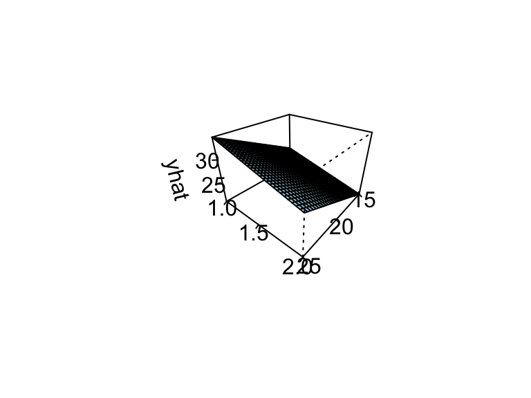
The regression model $$\begin{array}{rl}\hat{y}& =27.5+(\frac{8.33}{2})x_1+(\frac{-5.00}{2})x_2\end{array}$$ can be used generate response surface plots.

It is desirable to construct such plots on the natural factor levels than the coded factor levels, so $$\begin{array}{rl}\hat{y}& =27.5+(\frac{8.33}{2})(\frac{\text{Conc}-20}{5})+(\frac{-5.00}{2})(\frac{\text{Catalyst}-1.5}{0.5})\\ & =18.33+0.833\text{Conc}-5.00\text{Catalyst}\end{array}$$

---

res <- lm(y~A+B, data=dat)
res

Call:
lm(formula = y ~ A + B, data = dat)

Coefficients:
(Intercept)            A            B  
    18.3333       0.8333      -5.0000  

---

conc <- seq(15, 25, length=30)
cata <- seq(1, 2, length=30)
yhatn <- outer(conc, cata, function(x, y) 18.33 + .833*x - 5*y) 
persp(conc, cata, yhatn, theta=130, phi=30, expand=.7,
   zlab="\n\nyhat", xlab="", ylab="", nticks=3, 
col="lightblue",  ticktype="detailed")

---

contour(conc, cata, yhatn, nlevels=6, xlab="concentration",
        ylab="catalyst")

Example

A router is used to cut registration notches in printed circuit boards. The average notch dimension is satisfactory, but there is too much variability in the process. This excess variability leads to problems in board assembly. A quality control team assigned to this project decided to use a designed experiment to study the process. The team considered two factors: bit size ($A$) and speed ($B$).

Two levels were chosen for each factor (bit size $A$ at 1/16 inch and 1/8 inch and speed $B$ at 40 rpm and 80 rpm and a $2^2$ design was set up. Four boards were tested at each of the four runs in the experiment, and the resulting data are shown in the following table:

---

$$\overline{)\begin{array}{ccccccccr}Run& & \mathit{A}& \mathit{B}& & Vibration& & & \text{Total}\\ 1& (1)& -& -& 18.2& 18.9& 12.9& 14.4& 64.4\\ 2& a& +& -& 27.2& 24.0& 22.4& 22.5& 96.1\\ 3& b& -& +& 15.9& 14.5& 15.1& 14.2& 59.7\\ 4& ab& +& +& 41.0& 43.9& 36.3& 39.9& 161.1\end{array}}$$

1. Compute the main effects and interaction effect.
2. Compute the sum of squares associated with the effects.
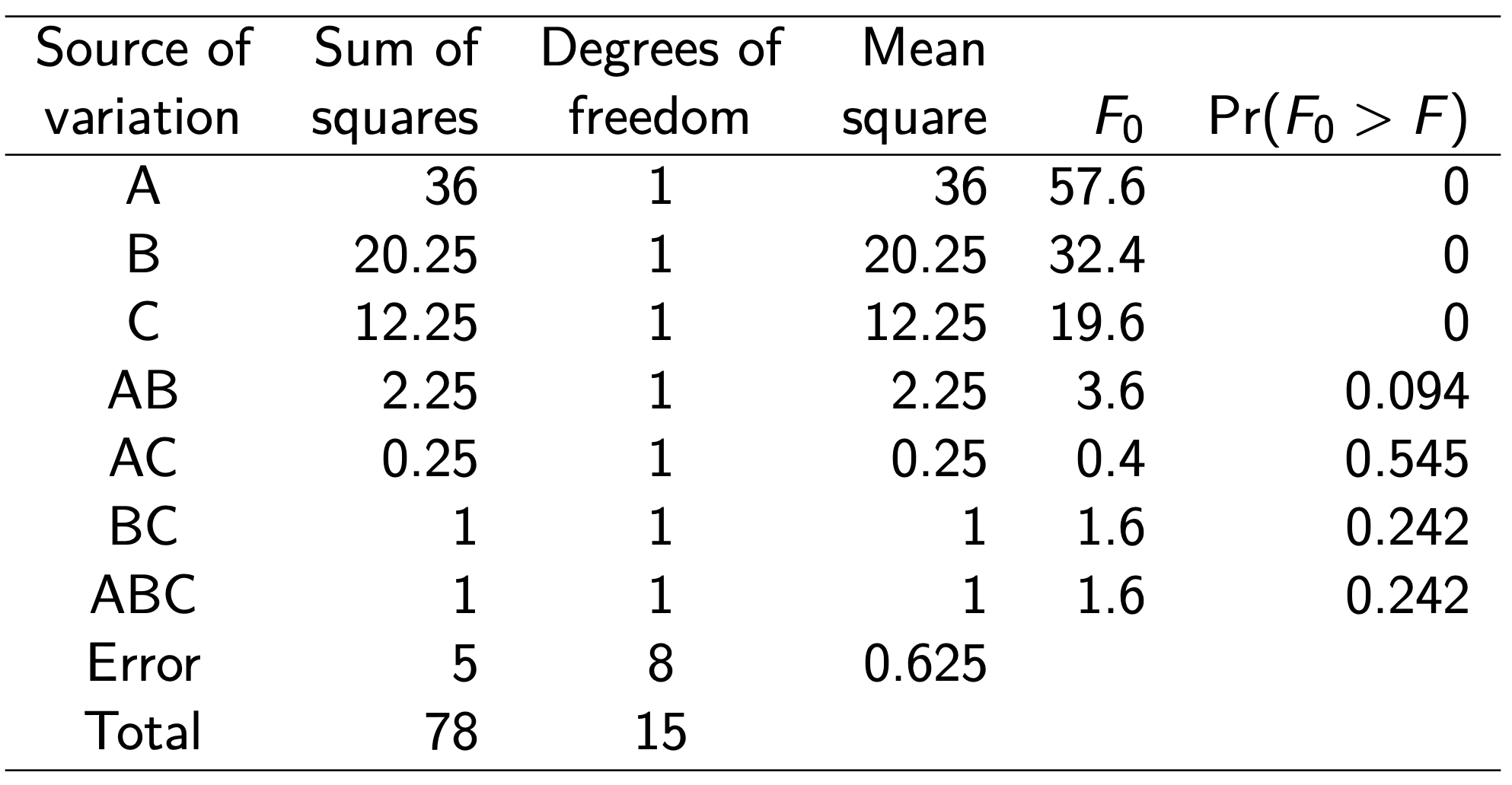
3. Construct the ANOVA table and draw conclusion.
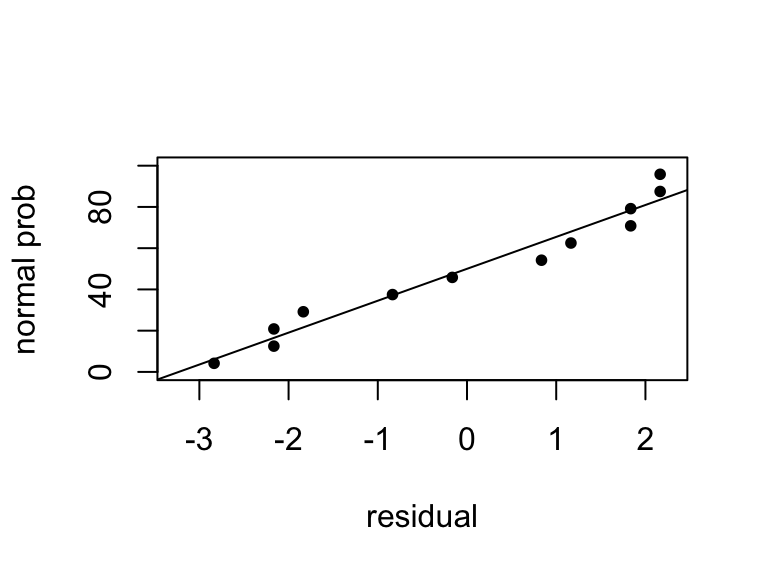
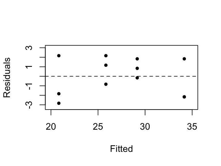
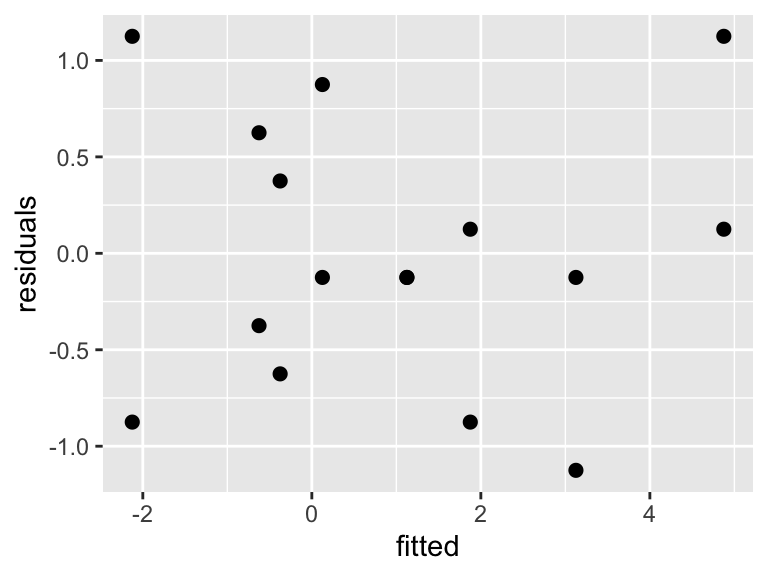
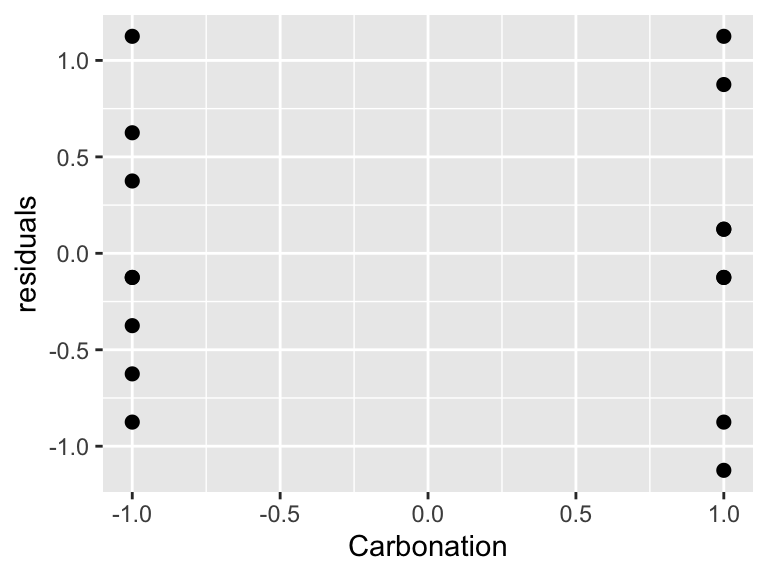
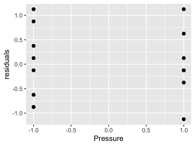
4. Find residuals using regression method.

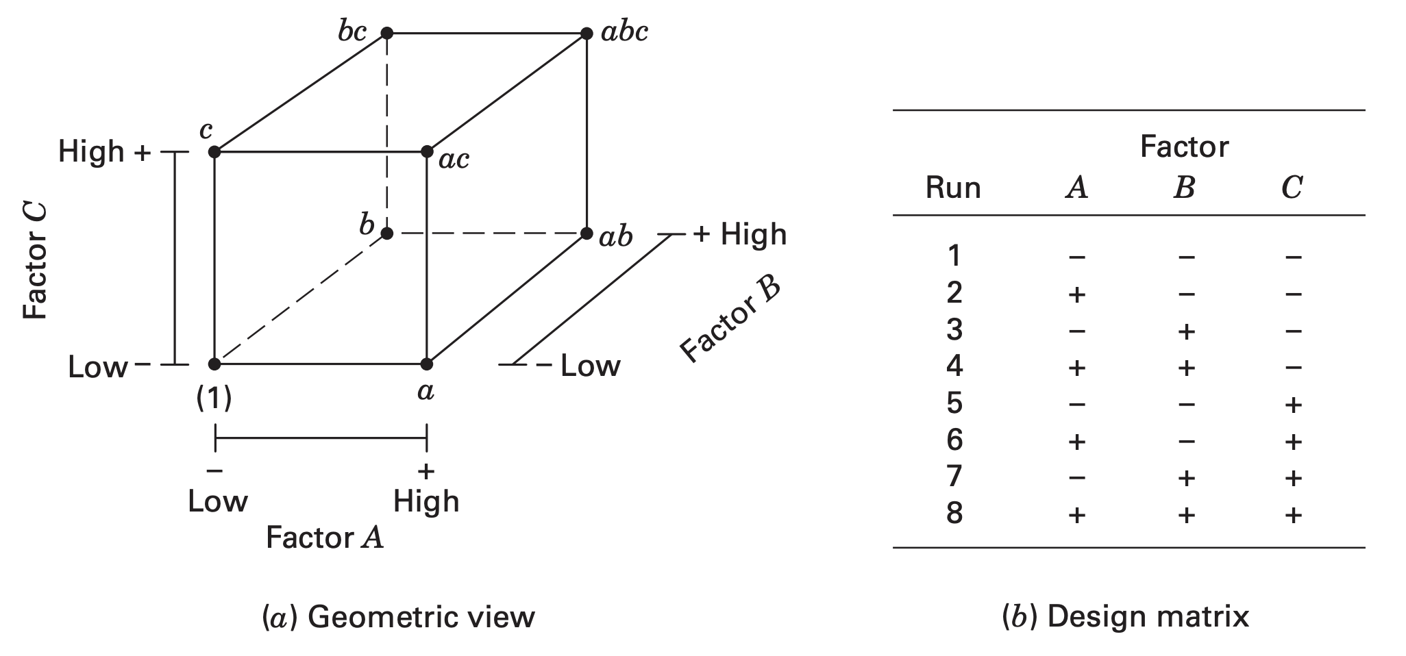
6.3 The $2^3$ design

The $2^3$ factorial design has three factors (say $A$, $B$, and $C$) and each factor has two levels each. The design has 8 treatment combinations.

---

• Standard order $\to$ $(1),a,b,ab,c,ac,bc$, and $abc$.
  • Remember that these symbols also represent the total of all $n$ observations taken at that particular treatment combination.
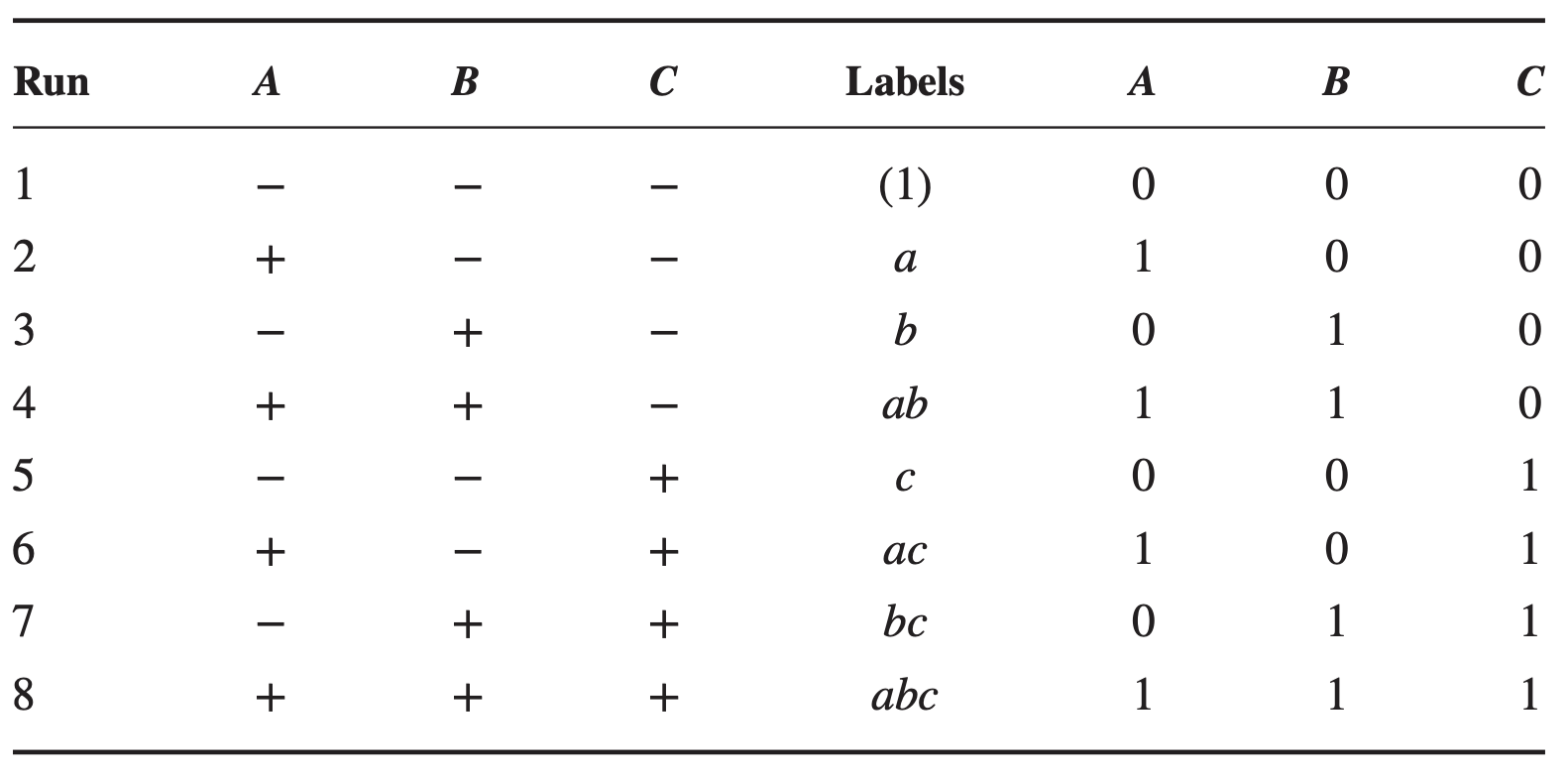
• Three different notations for $2^3$ design:

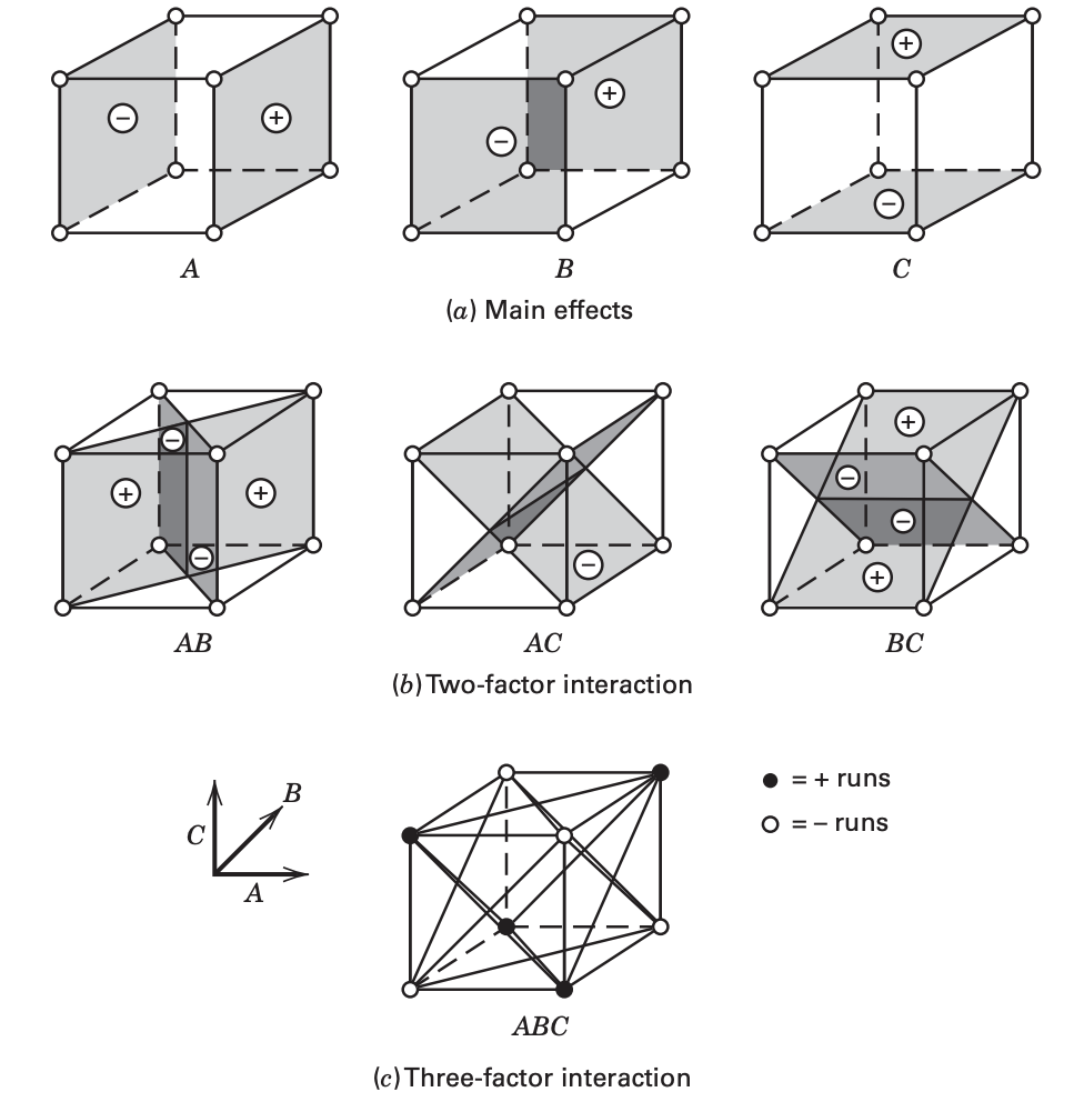
Effects in the $2^3$ design

• Main effects: $A$, $B$, and $C$

• Two-factor interactions: $AB$, $AC$, $BC$

• Three-factor interaction: $ABC$

---

---

The $A$ effect is just the average of the four runs where $A$ is at the high level $\left({\overline{y}}_{A^{+}}\right)$ minus the average of the four runs where $A$ is at the low level $\left({\overline{y}}_{A^{-}}\right)$, $$\begin{array}{rl}A& ={\overline{y}}_{A^{+}}-{\overline{y}}_{A^{-}}\\ & =\frac{a+ab+ac+abc}{4n}-\frac{(1)+b+c+bc}{4n}\end{array}$$

This equation can be rearranged as $$A=\frac{1}{4n}[a+ab+ac+abc-(1)-b-c-bc]$$

Similarly $$\begin{array}{rl}B& =\frac{1}{4n}[b+ab+bc+abc-(1)-a-c-ac]\\ C& =\frac{1}{4n}[c+ac+bc+abc-(1)-a-b-ab]\end{array}$$

The quantities in brackets are contrasts in the treatment combinations

Table of plus and minus signs for calculating effects

• The column for $A,B$, abd $C$ are actually from the design matrix.

• This table actually contains all the contrasts.

---

Construction of plus and minus table:

1. Signs for the main effects are determined by associating a plus with the high level and a minus with the low level.

2. Once the signs for the main effects have been established, the signs for the remaining columns can be obtained by multiplying the appropriate preceding columns

---

Interesting properties of Table of plus and minus signs:

1. Except the column $I$, every column has an equal number of $+$ and $-$ signs

2. The sum of the products of any two columns is zero

3. The column $I$ multiplied any column leaves the column unchanged, column $I$ is known as identity column

4. Product of any two columns yields a column in the table, e.g.  $A\times B=AB,AB\times BC=A{B}^{2}C=AC(\text{mod 2})$.

Exponents in the products are formed by using modulus 2 arithmetic.

Property-2 indicates that it is an Orthogonal design

Sum of squares

In the $2^3$ design with $n$ replicates, the sum of squares for any effect is $$SS=\frac{{\text{Contrast}}^2}{2^{3}n}=\frac{{\text{Contrast}}^2}{8n}$$

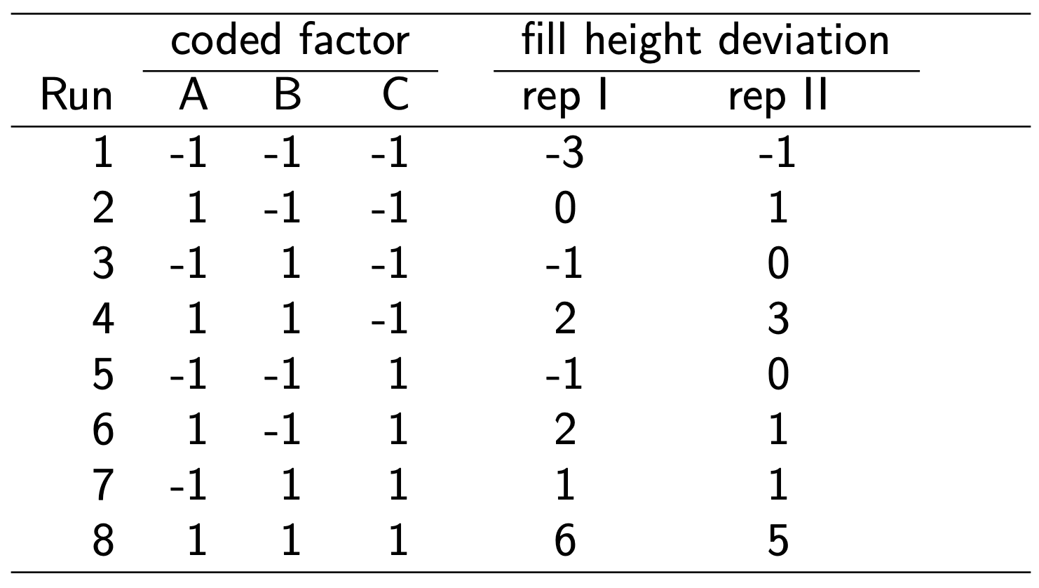
The $2^3$ design: An example

A soft drink bottler is interested in obtaining more uniform fill heights in the bottles produced his manufacturing process.

The filling machine theoretically fills fills each bottle to the correct target height, but in practice, there is variation around this target.

The bottler would like to understand better the sources of variability and eventually reduce it.

The process engineer can control three factors during the filling process: percentage of carbonation (A), operating pressure (B), and line speed (C).

Each factor has two levels: A (10% and 12%), B (25 psi and 30 psi), and C (200 b/min and 300 b/min).

---

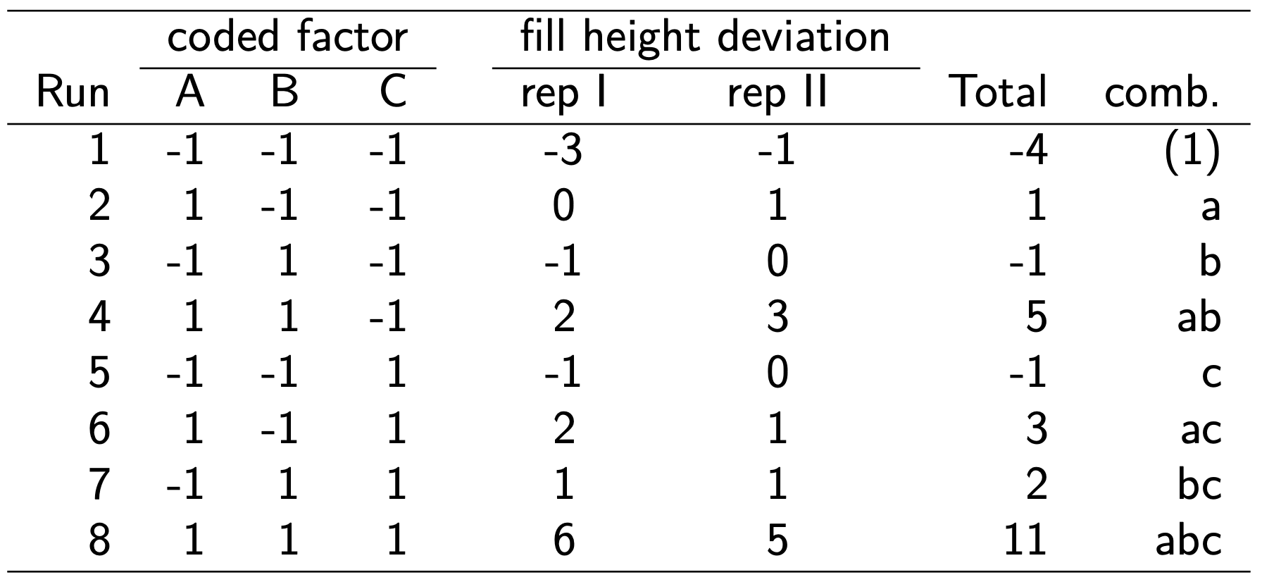
The data:

Notation for the response: $y_{ijkl},i,j,k,l=1,2$

---

Estimation of effects

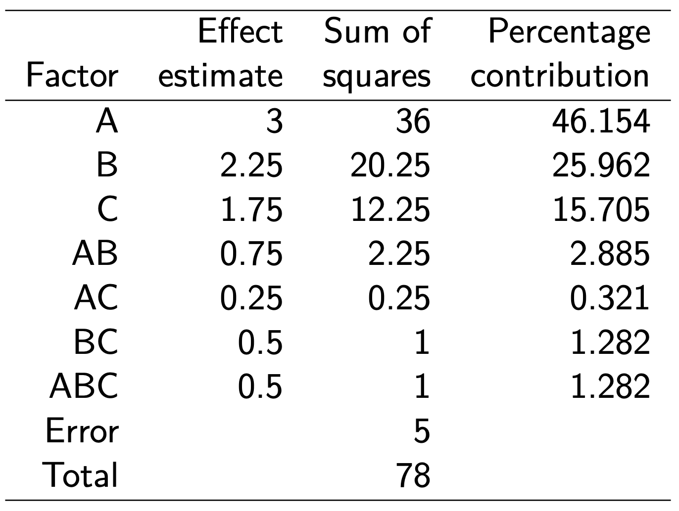
Main effect of A $$\begin{array}{rl}A& =(abc+ab+ac+a-bc-b-c-(1))/4n\\ & =(11+5+3+1-2+1+1+4)/8\\ & =24/8\\ & =3\end{array}$$ Similarly, $$\begin{array}{rl}B& =(abc+ab+bc+b-ac-a-c-(1))/4n=2.25\\ \\ C& =(abc+ac+bc+c-ab-a-b-(1))/4n=1.75\end{array}$$

---

Interactions $$\begin{array}{rl}AB& =(abc+ab+c+(1)-ac-bc-a-b)/4n=0.75\\ \\ AC& =(abc+ac+b+(1)-ab-bc-a-c)/4n=0.25\\ \\ BC& =(abc+bc+a+(1)-ab-ac-b-c)/4n=0.5\\ \\ ABC& =(abc+a+b+c-ab-ac-bc-(1))/4n=0.5\end{array}$$

Sum of squares

$$\begin{array}{rlrl}S{S}_A& =\frac{{\text{Contrast}}_A^2}{8n}=\frac{{24}^2}{16}=36& S{S}_{AB}& =\frac{6^2}{16}=2.25\\ \\ S{S}_B& =\frac{{18}^2}{16}=20.25& S{S}_{AC}& =\frac{2^2}{16}=0.25\\ \\ S{S}_C& =\frac{{14}^2}{16}=12.25& S{S}_{BC}& =\frac{4^2}{16}=1\\ \\ S{S}_{ABC}& =\frac{4^2}{16}=1& \end{array}$$

---

Percentage contribution is a rough but effective guide to the relative importance of each model term. Main effects dominate the process accounting for over 87 percent of the total variation.

Analysis of variance table

All the main effects are highly significant and only the interaction between carbonation and pressure is significant at about 10 percent level of significance.

Regression model

The fitted regression model for the design is $$\begin{array}{rl}\hat{y}& =1+(\frac{3}{2})x_A+(\frac{2.25}{2})x_B+(\frac{1.75}{2})x_C+(\frac{0.75}{2})x_A{x}_B\\ & =1+(\frac{3}{2})\frac{\text{carb}-11}{1.0}+(\frac{2.25}{2})\frac{\text{pres}-27.5}{2.5}+(\frac{1.75}{2})\frac{\text{speed}-250}{50}\\ & +(\frac{0.75}{2})(\frac{\text{carb}-11}{1.0})(\frac{\text{pres}-27.5}{2.5})\\ \\ \hat{y}& =9.625+2.62\text{carb}-1.20\text{pres}+0.035\text{speed}+0.38\text{carb}\times \text{speed}\end{array}$$

---

The model sum of squares is $$S{S}_{\text{Model }}=S{S}_A+S{S}_B+S{S}_C+S{S}_{AB}+S{S}_{AC}+S{S}_{BC}+S{S}_{ABC}$$

Thus the statistic $$F_0=\frac{M{S}_{\text{Model }}}{M{S}_E}$$ is testing the hypotheses $$H_0:{\beta }_1={\beta }_2={\beta }_3={\beta }_{12}={\beta }_{13}={\beta }_{23}={\beta }_{123}=0$$ $H_1$ : at least one $\beta \ne 0$

If ${\mathrm{F}}_0$ is large, we would conclude that at least one variable has a nonzero effect. Then each individual factorial effect is tested for significance using the $F$ statistic.

---

$$R^2=\frac{S{S}_{\text{Model }}}{S{S}_{\text{Total }}}$$ It measures the proportion of total variability explained by the model.

A potential problem with this statistic is that it always increases as factors are added to the model, even if these factors are not significant. The adjusted ${\mathrm{R}}^2$ statistic, defined as $$R_{\text{Adj }}^2=1-\frac{S{S}_E/d{f}_E}{S{S}_{\text{Total }}/d{f}_{\text{Total }}}$$

---

$R_{\text{Adj }}^2$ is a statistic that is adjusted for the “size” of the model, that is, the number of factors.

The adjusted ${\mathrm{R}}^2$ can actually decrease if nonsignificant terms are added to a model. The standard error of each coefficient, defined as $$se(\hat{\beta })=\sqrt{V(\hat{\beta })}=\sqrt{\frac{M{S}_E}{n{2}^k}}=\sqrt{\frac{M{S}_E}{N}}$$

---

The 95 percent confidence intervals on each regression coefficient are computed from $$\hat{\beta }-t_{0.025,N-p}\mathrm{se}(\hat{\beta })\le \beta \le \hat{\beta }+t_{0.025,N-p}\mathrm{se}(\hat{\beta })$$ where the degrees of freedom on $t$ are the number of degrees of freedom for error; that is, $N$ is the total number of runs in the experiment (16), and $p$ is the number of model parameters (8).

Other Methods for Judging the Significance of Effects.

The analysis of variance is a formal way to determine which factor effects are nonzero. Several other methods are useful. Now, we show how to calculate the standard error of the effects, and we use these standard errors to construct confidence intervals on the effects.

Confidence Interval of the Effect:

The $100(1-\alpha )$ percent confidence intervals on the effects are computed from $$\mathrm{Effect}\pm t_{\alpha /2,N-p}\ast \mathrm{se}(\mathrm{Effect}),$$ where $$se(\text{Effect})=\frac{2S}{\sqrt{n{2}^k}},\text{where}{S}^2=M{S}_E$$

Regression analysis with R

# Define the response variable
y3 <- c(-3, 0, -1, 2, -1, 2, 1, 6,
        -1, 1, 0, 3, 0, 1, 1, 5)

# Create treatment variables
xA <- rep(c(-1, 1), each = 1, times = 8)
xB <- rep(c(-1, 1), each = 2, times = 4)
xC <- rep(c(-1, 1), each = 4, times = 2)

# Fit the linear model
reg.y3 <- lm(y3 ~ xA + xB + xC + xA:xB)
coef(reg.y3)

(Intercept)          xA          xB          xC       xA:xB 
      1.000       1.500       1.125       0.875       0.375 

---

anova(reg.y3)

Analysis of Variance Table

Response: y3
          Df Sum Sq Mean Sq F value    Pr(>F)    
xA         1  36.00  36.000 54.6207 1.376e-05 ***
xB         1  20.25  20.250 30.7241 0.0001746 ***
xC         1  12.25  12.250 18.5862 0.0012327 ** 
xA:xB      1   2.25   2.250  3.4138 0.0916999 .  
Residuals 11   7.25   0.659                      
---
Signif. codes:  0 '***' 0.001 '**' 0.01 '*' 0.05 '.' 0.1 ' ' 1

Residual analysis

library(broom)
ggplot(augment(reg.y3)) +
  geom_point(aes(.fitted, .resid), size = 2) +
  labs(x = "fitted", y = "residuals")

---

ggplot(augment(reg.y3)) +
  geom_point(aes(xA, .resid), size = 2) +
  labs(x = "Carbonation", y = "residuals") 

---

ggplot(augment(reg.y3)) +
  geom_point(aes(xB, .resid), size = 2) +
  labs(x = "Pressure", y = "residuals") 

---

qqnorm(residuals(reg.y3))
qqline(residuals(reg.y3))

Full model vs our model

dat2 <- data.frame(y=y3, x1=xA, x2=xB, x3=xC)
head(dat2)

   y x1 x2 x3
1 -3 -1 -1 -1
2  0  1 -1 -1
3 -1 -1  1 -1
4  2  1  1 -1
5 -1 -1 -1  1
6  2  1 -1  1

---

res2 <- lm(y~xA*xB*xC, data=dat2)
anova(res2)

Analysis of Variance Table

Response: y
          Df Sum Sq Mean Sq F value    Pr(>F)    
xA         1  36.00  36.000    57.6 6.368e-05 ***
xB         1  20.25  20.250    32.4 0.0004585 ***
xC         1  12.25  12.250    19.6 0.0022053 ** 
xA:xB      1   2.25   2.250     3.6 0.0943498 .  
xA:xC      1   0.25   0.250     0.4 0.5447373    
xB:xC      1   1.00   1.000     1.6 0.2415040    
xA:xB:xC   1   1.00   1.000     1.6 0.2415040    
Residuals  8   5.00   0.625                      
---
Signif. codes:  0 '***' 0.001 '**' 0.01 '*' 0.05 '.' 0.1 ' ' 1

---

res3 <- lm(y~xA+xB+xC+xA:xB, data=dat2)
anova(res3)

Analysis of Variance Table

Response: y
          Df Sum Sq Mean Sq F value    Pr(>F)    
xA         1  36.00  36.000 54.6207 1.376e-05 ***
xB         1  20.25  20.250 30.7241 0.0001746 ***
xC         1  12.25  12.250 18.5862 0.0012327 ** 
xA:xB      1   2.25   2.250  3.4138 0.0916999 .  
Residuals 11   7.25   0.659                      
---
Signif. codes:  0 '***' 0.001 '**' 0.01 '*' 0.05 '.' 0.1 ' ' 1

---

anova(res3, res2)

Analysis of Variance Table

Model 1: y ~ xA + xB + xC + xA:xB
Model 2: y ~ xA * xB * xC
  Res.Df  RSS Df Sum of Sq   F Pr(>F)
1     11 7.25                        
2      8 5.00  3      2.25 1.2   0.37

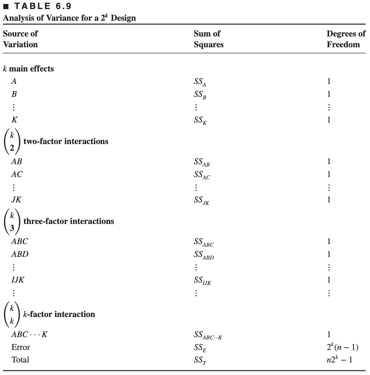
6.4 The general $2^k$ design

The general $2^k$ design

• The $2^k$ factorial design is a design with $k$ factors each has two levels.

• A statistical model for $2^k$ design would include

  • $k$ main effects
  • $(\genfrac{}{}{0ex}{}{k}{2})$ two-factor interactions
  • $(\genfrac{}{}{0ex}{}{k}{3})$ three-factor interactions
  • $\dots$
  • one $k$-factor interaction

• For a $2^k$ design, the complete model would contain $2^k-1$ effects

• The treatment combinations can be written in a standard order, e.g.
  $$(1)ababcacbcabcdad\cdots$$

---

• The complete model for $2^k$ design with $n$ replications has
  • $n{2}^k-1$ total degrees of freedom
  • $(n{2}^k-1)-(2^k-1)=2^k(n-1)$ error degrees of freedom
• For a $2^k$ design, contrast for the effect $AB\cdots K$ can be expressed as $${\text{Contrast}}_{AB\cdots }=(a\pm 1)(b\pm 1)\cdots (k\pm 1)$$
  • ordinary algebra is used with “1” being replaced by (1) in the final expression.
  • The sign in each set of parentheses is negative if the factor is included in the effect and positive if the factor is not included.
• E.g. for a $2^2$ design, the contrast $$\begin{array}{rl}A& =(a-1)(b+1)=ab+a-b-(1)\\ AB& =(a-1)(b-1)=ab-a-b+(1)\end{array}$$

---

• Estimate of the contrast $$AB\dots K=\frac{2}{n{2}^k}[{\text{Contrast}}_{AB\cdots K}]$$

• Sums of squares $$S{S}_{AB\dots K}=\frac{1}{n{2}^k}[{\text{Contrast}}_{AB\cdots K}{]}^2,$$ where $n$ is the number of replications.

---

---

6.5 A single replicate of the $2^k$ design

• Total number of treatment combinations in a $2^k$ factorial design could be very large even for a moderate number of factors

• For example, a $2^5$ design has 32 treatment combinations, a $2^6$ design has 64 treatment combinations, and so on

• In many practical situations, the available resources may only allow a single replicate of the design to be run

• Single replicate may cause problem if the response is highly variable

• A single replicate of a $2^k$ design is sometime called an unreplicated factorial

---

• With only one replicate, pure error cannot be estimated, so commonly used analysis of variance cannot be performed

• Two approaches are commonly used for analysing unreplicated factorial design

1. Consider certain high-order interactions as negligible and combine their mean squares to estimate the error.
   • This approach is based on the assumption that the most systems is dominated by some of the main effects and low-order interactions, and most of the high-order interactions are negligible (sparsity of effects principle)

---

2. Higher-order interactions could be of interest, in that case polling higher-order interactions to estimate the error variance is not appropriate.
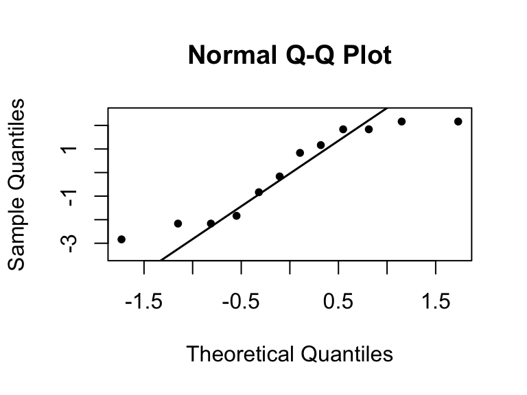
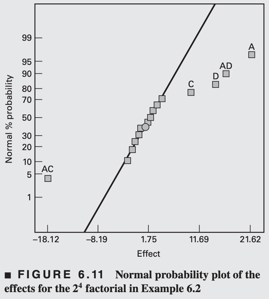
   • In such case, normal probability plots of the effect estimates could be of help. The negligible effects should be normally distributed with mean 0 and variance ${\sigma }^2$ and will fall in a straight line on the plot. On the other hand, significant effects will have nonzero means and will not lie along the straight line.

---

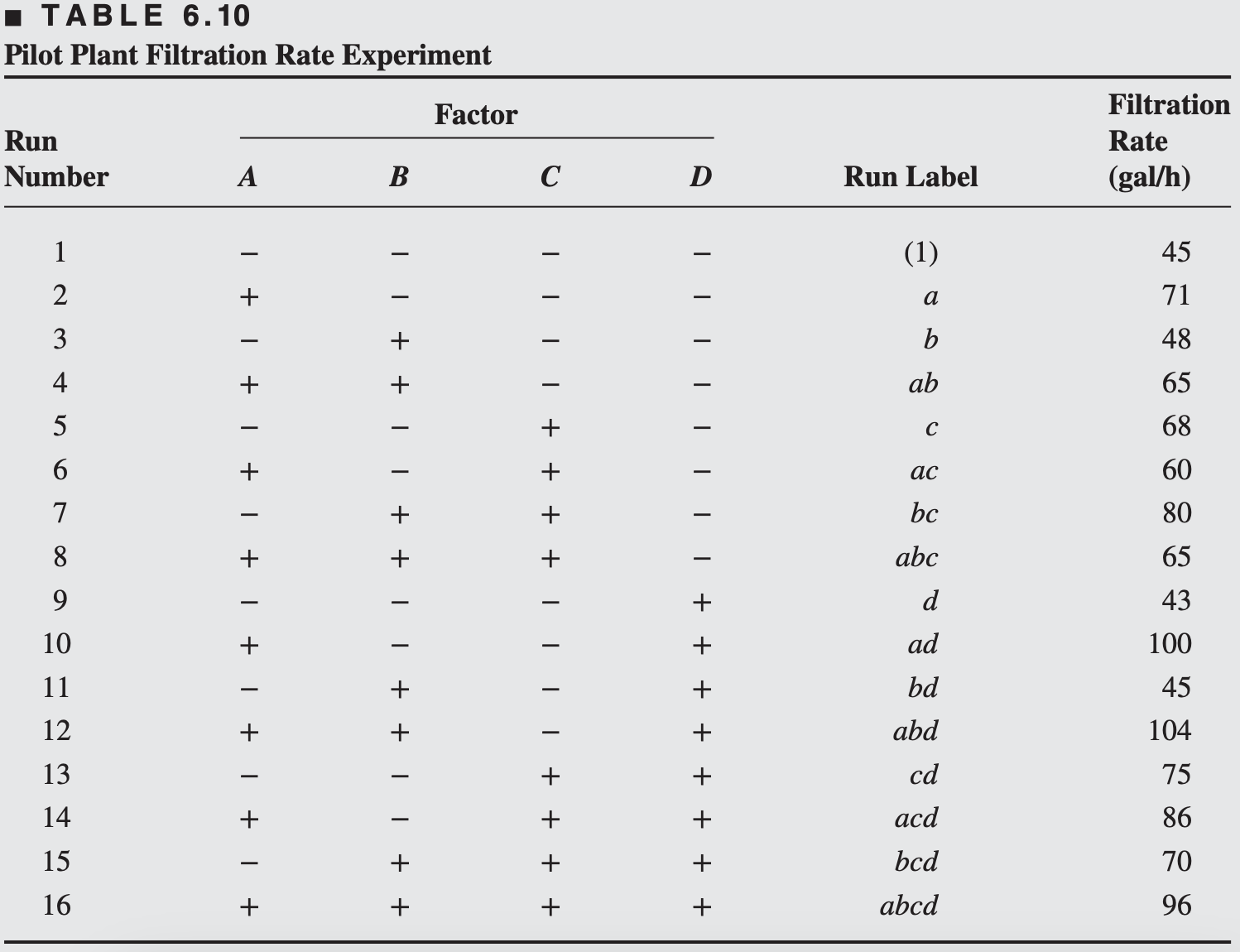
EXAMPLE 6.2

A chemical product is produced in a pressure vessel. A factorial experiment is carried out in the pilot plant to study the factors thought to influence the filtration rate of this product.

Four factors temperature (A), pressure (B), concentration of formaldehyde (C), and stirring rate (D) are thought to be important for the chemical product.

The design matrix and the response data obtained from a single replicate of the $2^4$ experiment are shown in Table 6.10.

---

---

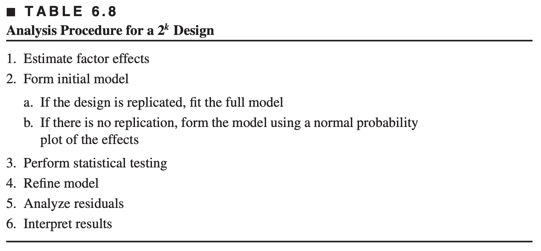
• We will begin the analysis of these data by constructing a normal probability plot of the effect estimates.

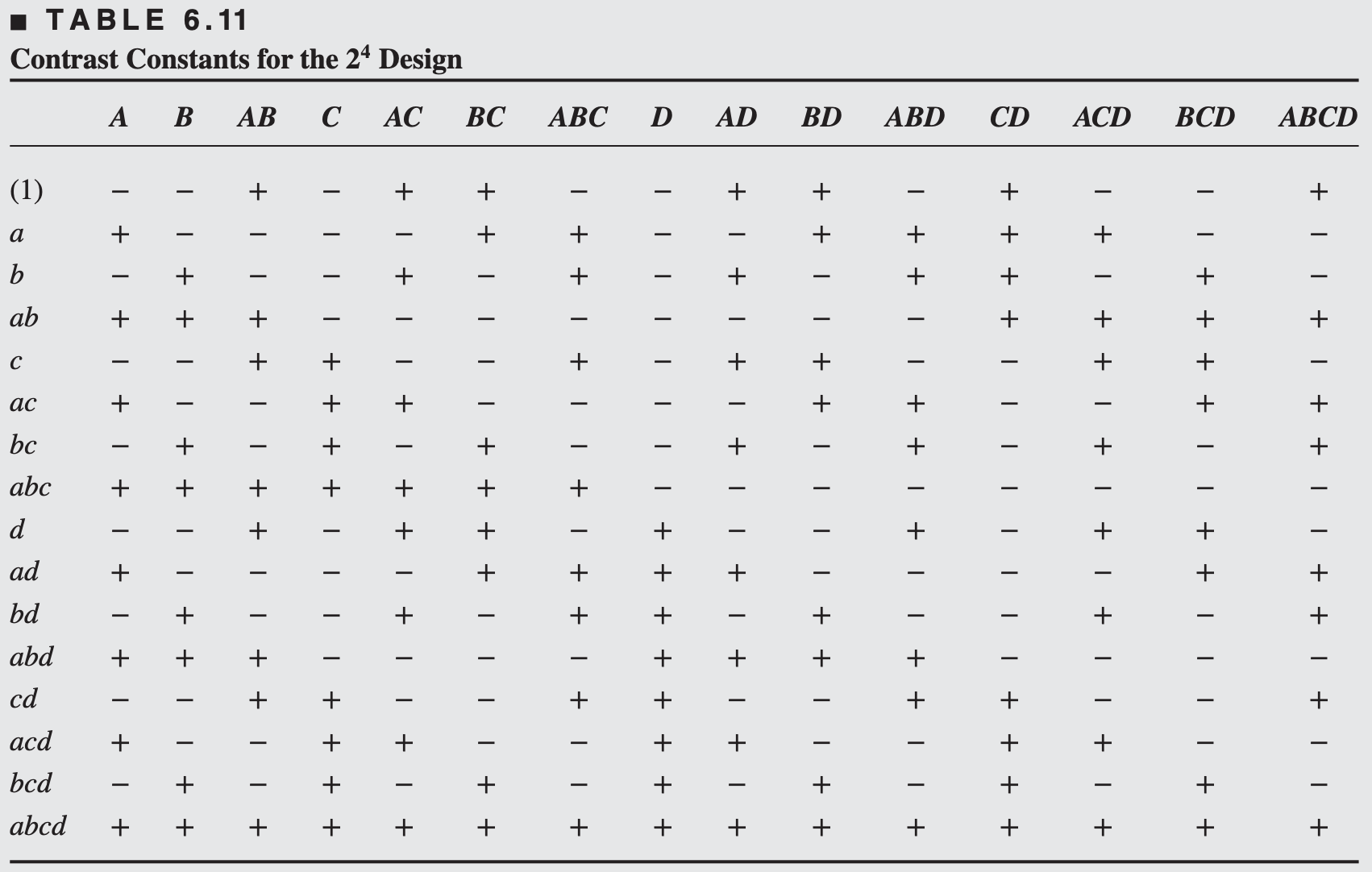
  • The table of plus and minus signs for the contrast constants for the $2^4$ design are shown in Table 6.11.

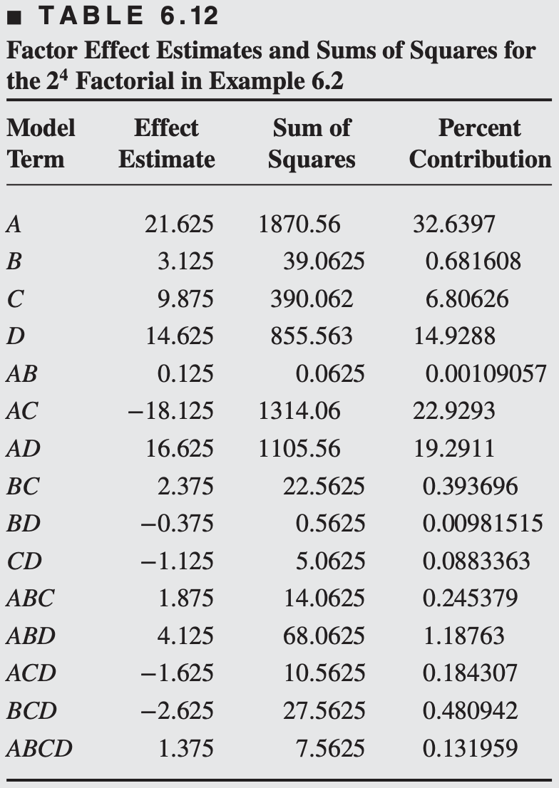
  • From these contrasts, we may estimate the 15 factorial effects and the sums of squares shown in Table 6.12.

---

---

---

df <- data.frame(
  y  = c(45, 71, 48, 65, 68, 60, 80, 65, 43, 100, 45, 104, 75, 86, 70, 96),
  A = rep(c(-1, 1), times = 8),
  B = rep(c(-1, 1), each = 2, times = 4),
  C = rep(c(-1, 1), each = 4, times = 2),
  D = rep(c(-1, 1), each = 8)
)
model <- lm(y ~ A * B * C * D, data = df)
dat6b <- tibble(
  `Model terms` = c('A', 'B', 'C', 'D', 'AB', 'AC', 'BC',
                    'AD', 'BD', 'CD', 'ABC', 'ABD', 
                    'ACD', 'BCD', 'ABCD'),
  `Effect estimates` = coef(model)[-1] * 2,
   SS = anova(model)$"Sum Sq"[1:15],
  `Percentage contribution` = 100 * (SS / sum(SS))
)

---

kableExtra::kable(dat6b, digits = 3, align = 'c')

Model terms	Effect estimates	SS	Percentage contribution
A	21.625	1870.562	32.640
B	3.125	39.062	0.682
C	9.875	390.063	6.806
D	14.625	855.563	14.929
AB	0.125	0.062	0.001
AC	-18.125	1314.062	22.929
BC	2.375	22.562	0.394
AD	16.625	1105.562	19.291
BD	-0.375	0.563	0.010
CD	-1.125	5.063	0.088
ABC	1.875	14.063	0.245
ABD	4.125	68.062	1.188
ACD	-1.625	10.563	0.184
BCD	-2.625	27.563	0.481
ABCD	1.375	7.563	0.132

---

• The important effects that emerge from this analysis are

  • the main effects of $A,C,$ and $D$ and

  • the $AC$ and $AD$ interactions.

---

library(ggDoE)
main_effects(df, response='y', exclude_vars = c('B'),
             color_palette = 'viridis', n_columns=3)

Main effect plots

---

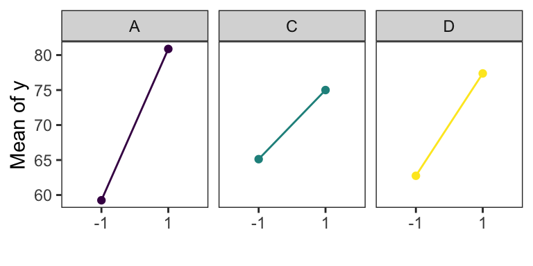
• The main effects of A, C, and D are plotted in Figure. All three effects are positive, and if we considered only these main effects, we would run all three factors at the high level to maximize the filtration rate.

• However, it is always necessary to examine any interactions that are important. Remember that main effects do not have much meaning when they are involved in significant interactions.

---

p1=interaction_effects(df, response='y',exclude_vars=c('B','D'))
p2=interaction_effects(df, response='y',exclude_vars=c('B','C'))
gridExtra::grid.arrange(p1, p2, ncol = 2)

Interaction plots

---

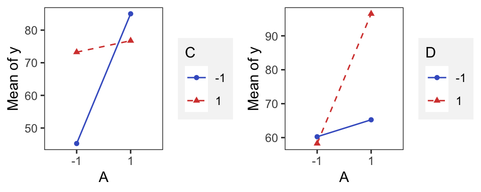
The AC interaction indictates: the $A$ effect is very small when the $C$ is at the high level and very large when the $C$ is at the low level, with the best results obtained with low C and high A.

The AD interaction indicates: $D$ has little effect at low $A$ but a large positive effect at high $A$.

Therefore, the best filtration rates would appear to be obtained when A and D are at the high level and C is at the low level. This would allow the reduction of the formaldehyde concentration to a lower level, another objective of the experimenter.

Design projection

• Another interpretation of the effects in Figure 6.11 is possible

• Because $B$ (pressure) is not significant and all interactions involving $B$ are negligible, we may discard $B$ from the experiment so that the design becomes a $2^3$ factorial in $A,C,$ and $D$ with two replicates.

• This is easily seen from examining only columns $A,C,$ and $D$ in the design matrix shown in Table 6.10 and noting that those columns form two replicates of a $2^3$ design.

---

---

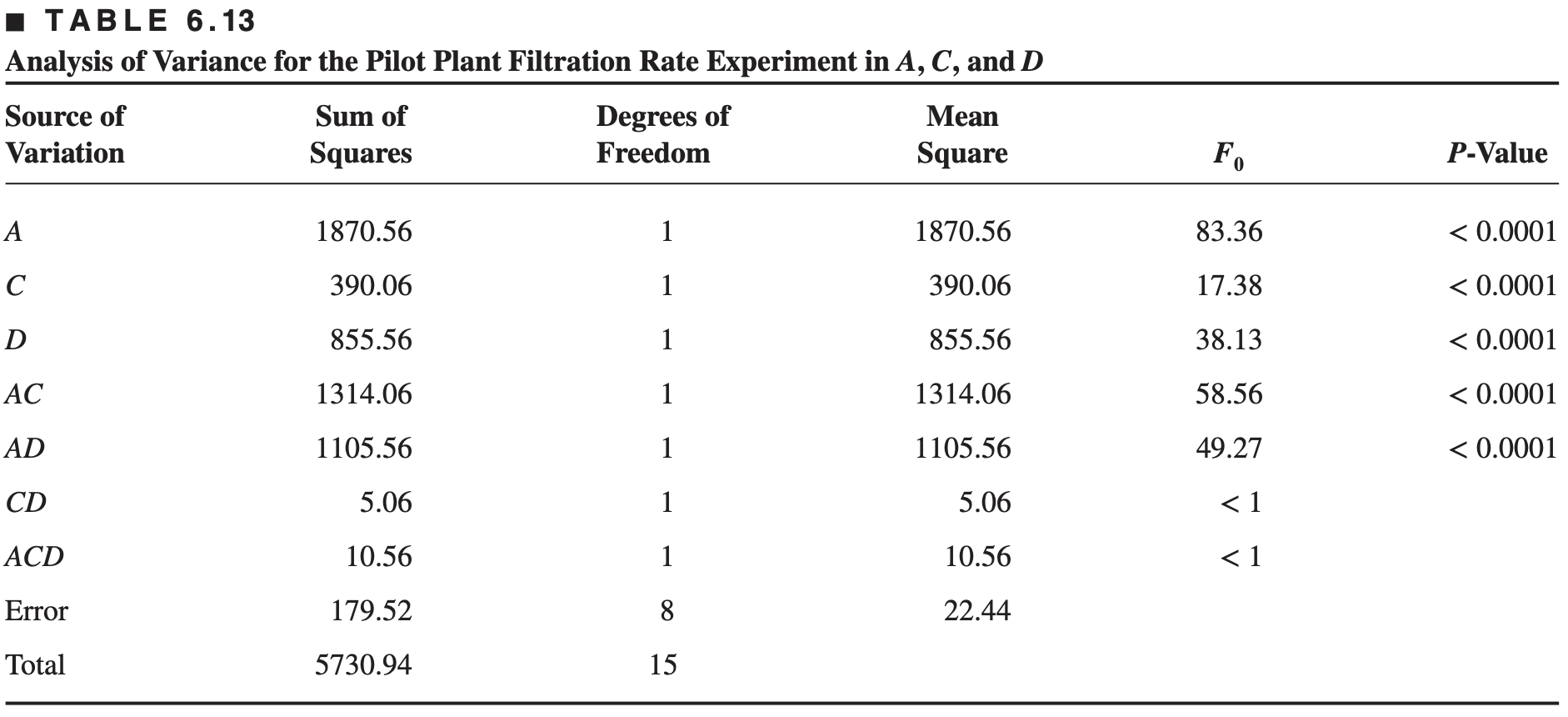
The analysis of variance for the data using this simplifying assumption is summarized in Table 6.13.

The conclusions that we would draw from this analysis are essentially unchanged from those of Example 6.2.

Note that by projecting the single replicate of the $2^4$ into a replicated $2^3$ , we now have both an estimate of the $ACD$ interaction and an estimate of error based on what is sometimes called hidden replication

In general, if we have a single replicate of a $2^k$ design, and if $h(h<k)$ factors are negligible and can be dropped, then the original data correspond to a full two-level factorial in the remaining $k-h$ factors with $2^h$ replicates.

---

The Half-Normal Plot of Effects

• An alternative to the normal probability plot of the factor effects is the half-normal plot.

• This is a plot of the absolute value of the effect estimates against their cumulative normal probabilities.

• The straight line on the half-normal plot always passes through the origin and should also pass close to the fiftieth percentile data value.

---

ggDoE::half_normal(model)

Other Methods for Analyzing Unreplicated Factorials.

A widely used analysis procedure for an unreplicated two-level factorial design is the normal (or half-normal) plot of the estimated factor effects.

However, unreplicated designs are so widely used in practice that many formal analysis procedures have been proposed to overcome the subjectivity of the normal probability plot.

Hamada and Balakrishnan (1998) compared some of these methods.

• They found that the method proposed by Lenth (1989) has good power to detect significant effects. It is also easy to implement, and as a result it appears in several software packages for analyzing data from unreplicated factorials.

6.6 Additional Examples of Unreplicated $2^k$ Designs

EXAMPLE 6.3: Data Transformation in a Factorial Design

6.7 $2^k$ Designs are Optimal Designs

The model parameter regression coefficients (and effect estimates) from a $2^k$ design are least squares estimates. For a $2^2$ model, the regression model is $$y={\beta }_0+{\beta }_1{x}_1+{\beta }_2{x}_2+{\beta }_{12}{x}_1{x}_2+\epsilon$$

The four observations from a $2^2$ design: $$\begin{array}{rl}& (1)={\beta }_0+{\beta }_1(-1)+{\beta }_2(-1)+{\beta }_{12}(-1)(-1)+{\epsilon }_1\\ & a={\beta }_0+{\beta }_1(1)+{\beta }_2(-1)+{\beta }_{12}(1)(-1)+{\epsilon }_2\\ & b={\beta }_0+{\beta }_1(-1)+{\beta }_2(1)+{\beta }_{12}(-1)(1)+{\epsilon }_3\\ & ab={\beta }_0+{\beta }_1(1)+{\beta }_2(1)+{\beta }_{12}(1)(1)+{\epsilon }_1\end{array}$$

$$\begin{array}{rl}& \mathbf{y}=\mathbf{X}\mathit{\beta }+\mathit{\epsilon },\mathbf{y}=\left[\begin{array}{c}(1)\\ a\\ b\\ ab\end{array}\right],\mathbf{X}=\left[\begin{array}{cccc}1& -1& -1& 1\\ 1& 1& -1& -1\\ 1& -1& 1& -1\\ 1& 1& 1& 1\end{array}\right],\mathit{\beta }=\left[\begin{array}{c}{\beta }_0\\ {\beta }_1\\ {\beta }_2\\ {\beta }_{12}\end{array}\right],\mathit{\epsilon }=\left[\begin{array}{c}{\epsilon }_1\\ {\epsilon }_2\\ {\epsilon }_3\\ {\epsilon }_4\end{array}\right]\end{array}$$

---

The least squares estimate of $\beta$ is given by: $$\hat{\beta }=(X^{\prime }X{)}^{-1}{X}^{\prime }y$$

Since this is an orthogonal design, the $X^{\prime }X$ matrix is diagonal:

$$\hat{\beta }={\left[\begin{array}{cccc}4& 0& 0& 0\\ 0& 4& 0& 0\\ 0& 0& 4& 0\\ 0& 0& 0& 4\end{array}\right]}^{-1}\left[\begin{array}{c}(1)+a+b+ab\\ a+ab-b-(1)\\ b+ab-a-(1)\\ (1)-a-b+ab\end{array}\right]$$

---

With this, we obtain:

$$\left[\begin{array}{c}{\hat{\beta }}_0\\ {\hat{\beta }}_1\\ {\hat{\beta }}_2\\ {\hat{\beta }}_{12}\end{array}\right]=\frac{1}{4}{\mathbf{I}}_4\left[\begin{array}{c}(1)+a+b+ab\\ a+ab-b-(1)\\ b+ab-a-(1)\\ (1)-a-b+ab\end{array}\right]=\left[\begin{array}{c}\frac{(1)+a+b+ab}{4}\\ \frac{a+ab-b-(1)}{4}\\ \frac{b+ab-a-(1)}{4}\\ \frac{(1)-a-b+ab}{4}\end{array}\right]$$

• The “usual” contrasts are shown in the matrix of $X^{\prime }y$.
• The $X^{\prime }X$ matrix is diagonal as a consequence of the orthogonal design.
• The regression coefficient estimates are exactly half of the “usual” effect estimates.

---

The matrix (X’X) has some useful properties

$$\begin{array}{rl}V(\hat{\beta })& ={\sigma }^2(\text{diagonal element of }(X^{\prime }X{)}^{-1})\\ & =\frac{{\sigma }^2}{4}⟶\text{Minimum possible value for a four-run design}\end{array}$$

$$|X^{\prime }X|=256⟶\text{Maximum possible value for a four-run design}$$

Notice that these results depend on both the design you have chosen and the model.

---

It turns out that the volume of the joint confidence region that contains all the model regression coefficients is inversely proportional to the square root of the determinant of $X\prime X$.

Therefore, to make this joint confidence region as small as possible, we would want to choose a design that makes the determinant of $X\prime X$ as large as possible.

In general, a design that minimizes the variance of the model regression coefficients (or maximize the determinant of $X\prime X$) is called a $D$-optimal design.

The $2^k$ design is a $D$-optimal design for fitting the first-order model or the first-order model with interaction.

6.8 The Addition of Center Points to the $2^k$ Design

A potential concern in the use of two-level factorial designs is the assumption of linearity in the factor effects.

First-order model (with interaction): $$y={\beta }_0+\sum _{j=1}^k{\beta }_j{x}_j+\sum \sum _{i<j}{\beta }_{ij}{x}_i{x}_j+ϵ.(6.28)$$ is capable of representing some curvature in the response function.

Second-order model: $$y={\beta }_0+\sum _{j=1}^k{\beta }_j{x}_j+\sum _{i<j}{\beta }_{ij}{x}_i{x}_j+\sum _{j=1}^k{\beta }_{ij}{x}_j^2+ϵ(6.29)$$ where ${\beta }_{jj}$ represent pure Second-order or quadratic effects.

---

In running a two-level factorial experiment, we usually anticipate fitting the first-order model in Equation 6.28, but we should be alert to the possibility that the second-order model in Equation 6.29 is more appropriate.

There is a method of replicating certain points in a $2^k$ factorial that will provide protection against curvature from second-order effects as well as allow an independent estimate of error to be obtained.

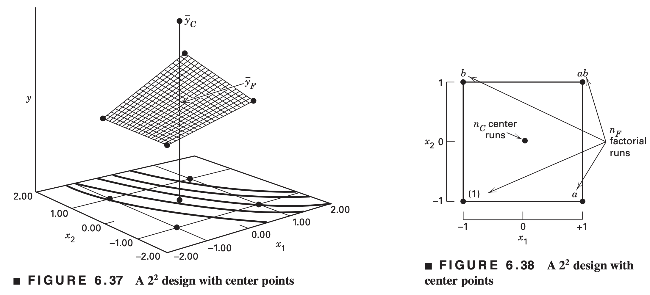
The method consists of adding center points to the $2^k$ design. These consist of $n_C$ replicates run at the points $x_i=0(i=1,2,\dots ,k)$.

One important reason for adding the replicate runs at the design center is that center points do not affect the usual effect estimates in a $2^k$ design.

When we add center points, we assume that the $k$ factors are quantitative.

---

---

Let ${\overline{y}}_F$ be the average of the $n_F$ runs at the four factorial points, and ${\overline{y}}_C$ be the average of the $n_C$ runs at the center point.

${\overline{y}}_F$ = ${\overline{y}}_C$ $\to$ no “curvature” $$\begin{array}{rl}& H_0:\sum _{j=1}^k{\beta }_{jj}=0\\ & H_1:\sum _{j=1}^k{\beta }_{jj}\ne 0\end{array}$$ $$S{S}_{\text{Pure quadratic }}=\frac{n_F{n}_C{({\overline{y}}_F-{\overline{y}}_C)}^2}{n_F+n_C}(6.30)$$ The sum of square has a single degree of freedom.

---

This sum of squares may be incorporated into the ANOVA and may be compared to the error mean square to test for pure quadratic curvature.

Furthermore, if the factorial points in the design are unreplicated, one may use the $n_C$ center points to construct an estimate of error with $n_C-1$ degrees of freedom.

Example 6.7 (Extended 6.2)

We will illustrate the addition of center points to a $2^k$ design by reconsidering the pilot plant experiment in Example 6.2.

Recall that this is an unreplicated $2^4$ design.

Refer to the original experiment shown in Table 6.10.

---

---

Suppose that four center points are added to this experiment, and at the points $x_1=x_2=x_3=x_4=0$ the four observed filtration rates were $73,75,66$, and $69$.

• The average of these four center points is ${\overline{y}}_C=70.75$
• The average of the 16 factorial runs is ${\overline{y}}_F=70.06$.

Since ${\overline{y}}_C$ and ${\overline{y}}_F$ are very similar, we suspect that there is no strong curvature present.

---

The mean square for pure error is calculated from the center points as follows: $$\begin{array}{rl}M{S}_E=\frac{S{S}_E}{n_C-1}& =\frac{\sum _{\text{Center points }}{(y_i-{\overline{y}}_c)}^2}{n_C-1}\\ & =\frac{\sum _{i=1}^4{(y_i-70.75)}^2}{4-1}=16.25\end{array}$$

---

The difference ${\overline{y}}_F-{\overline{y}}_C=70.06-70.75=-0.69$ is used to compute the pure quadratic (curvature) sum of squares from Equation 6.30 as follows: $$\begin{array}{rl}S{S}_{\text{Pure quadratic }}& =\frac{n_F{n}_C{({\overline{y}}_F-{\overline{y}}_C)}^2}{n_F+n_C}\\ & =\frac{(16)(4)(-0.69{)}^2}{16+4}=1.51\end{array}$$

---

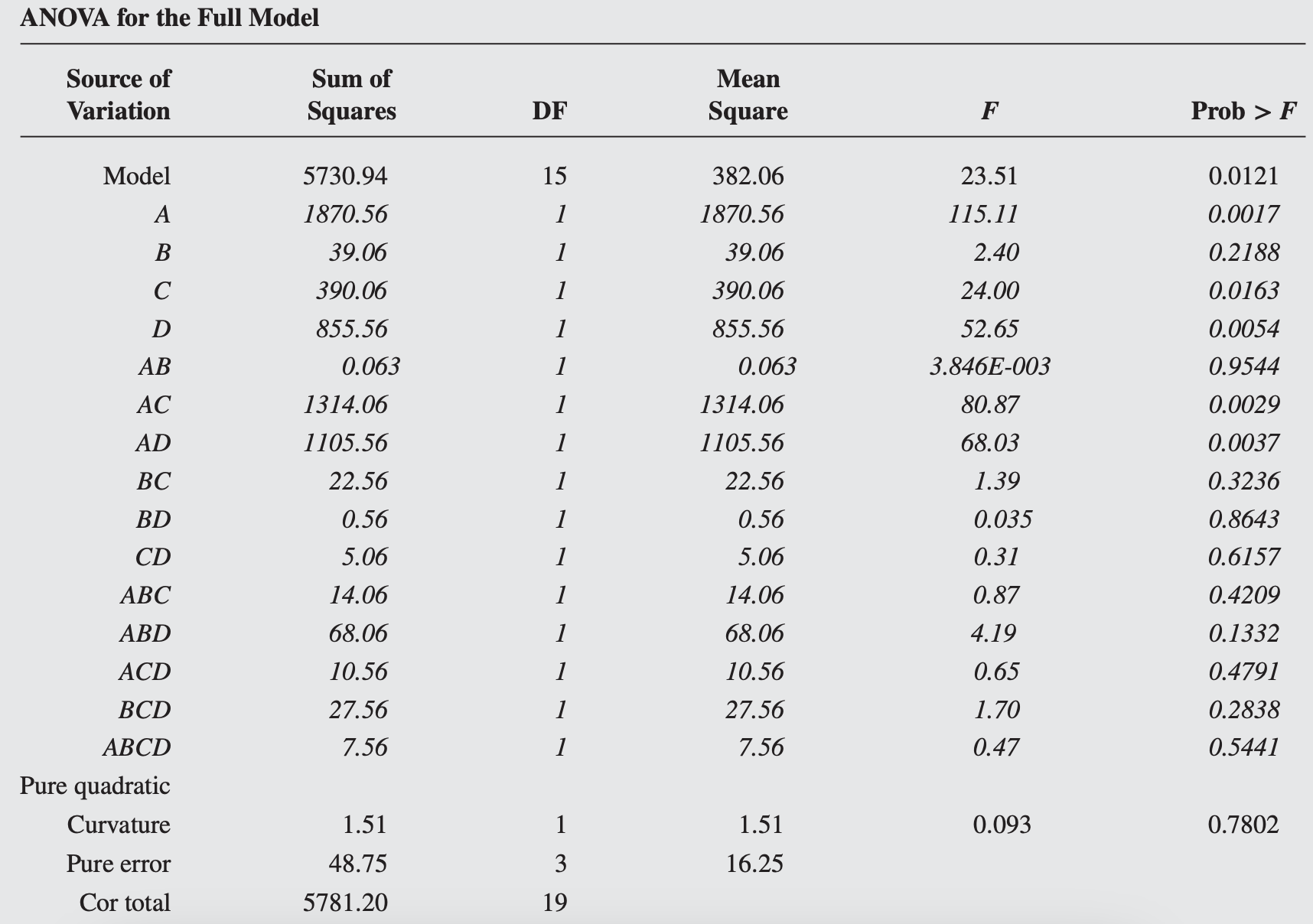
The upper portion of the Table 6.24 shows ANOVA for the full model.

---

The ANOVA indicates that there is no evidence of second-order curvature in the response over the region of exploration (p-value=0.7802).

That is, the null hypothesis $H_0:{\beta }_{11}+{\beta }_{22}+$ ${\beta }_{33}+{\beta }_{44}=0$ cannot be rejected.

The significant effects are $A,C,D,AC$, and $AD$.

---

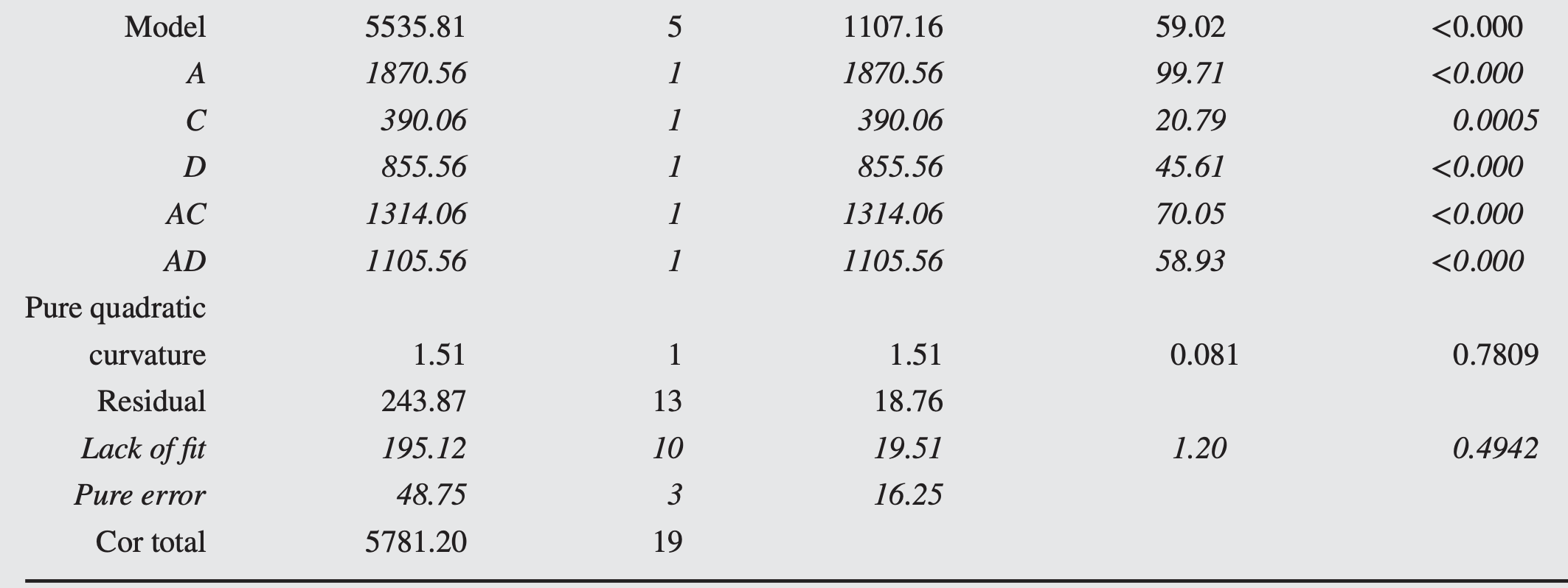
The ANOVA for the reduced model is shown in the lower portion of Table 6.24.

The results of this analysis agree with those from Example 6.2, where the important effects were isolated using the normal probability plotting method.