Chapter 5

(AST301) Design and Analysis of Experiments II

Author

Md Rasel Biswas

5 Introduction to Factorial Designs

5.1 Basic Definitions and Principles

Factorial design

Factorial designs deal with the experiments that involve the study of two or more factors.
In factorial design, all possible combinations of the levels of the factors are investigated in each complete replication.
- E.g. if there are $a$ levels of factor ${A}$ and $b$ levels of factor ${B}$, each replicate contains all $a b$ treatment combinations.
The effect of a factor is defined to be the change in response produced by a change in the level of the factor.
This is frequently called a main effect because it refers to the primary factors of interest in the experiment.

Example 5.1

For example, consider the simple experiment in Figure 5.1.
This is a two-factor factorial experiment with both design factors at two levels. We have called these levels “low” and “high” and denoted them “−” and “+,” respectively.

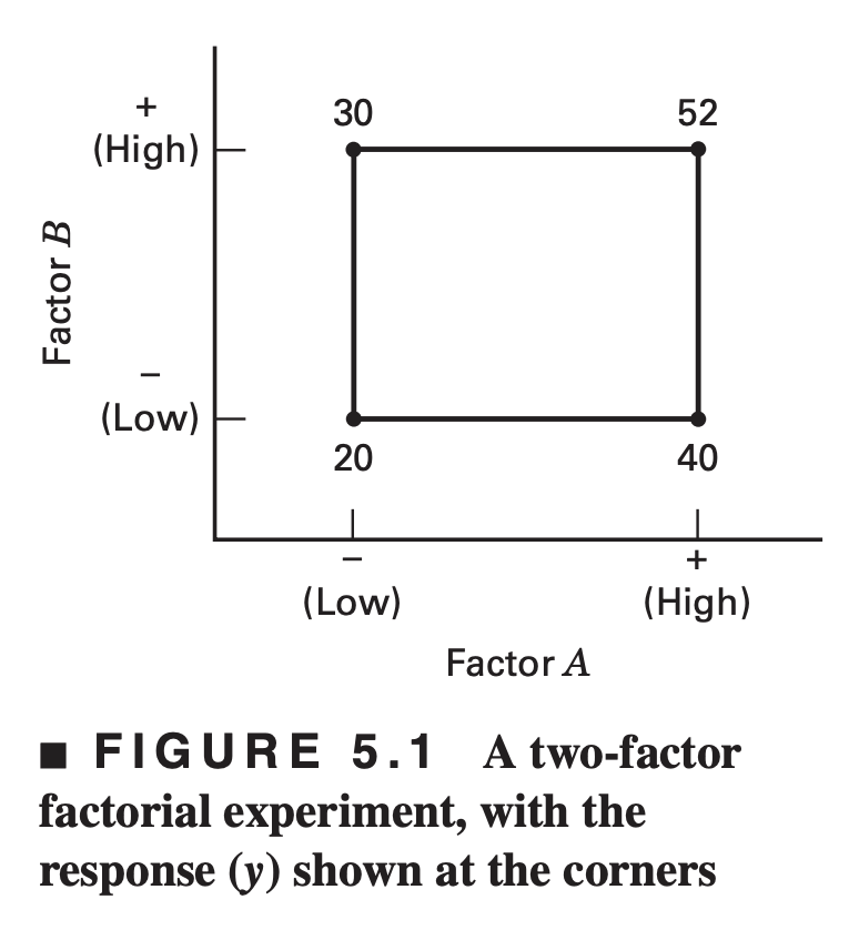
The main effect of factor $A$ in this two-level design can be thought of as the difference between the average response at the low level of $A$ and the average response at the high level of $A$. Numerically, this is \[ A=\frac{40+52}{2}-\frac{20+30}{2}=21 \]
That is, increasing factor $A$ from the low level to the high level causes an average response increase of 21 units
Similarly, the main effect of $B$ is \[ B=\frac{30+52}{2}-\frac{20+40}{2}=11 \]
If the factors appear at more than two levels, the above procedure must be modified because there are other ways to define the effect of a factor. This point is discussed more completely later.

Example 5.2

In some experiments, we may find that the difference in response between the levels of one factor is not the same at all levels of the other factors.
When this occurs, there is an interaction between the factors. For example, consider the two-factor factorial experiment shown in Figure 5.2

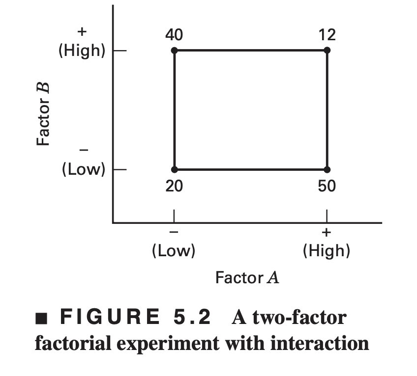
At the low level of factor $B$ (or $B−$), the $A$ effect is \[A = 50 − 20 = 30\]
At the high level of factor $B$ (or $B+$), the $A$ effect is \[A = 12 − 40 = −28\]
Because the effect of $A$ depends on the level chosen for factor $B$, we see that there is interaction between $A$ and $B$.
The magnitude of the interaction effect is the average difference in these two $A$ effects, or $AB = (−28 − 30)∕2 = −29$.
Clearly, the interaction is large in this experiment.

An interaction is the failure of one factor to produce the same effect on the response at different levels of another factor.

Illustrating interaction

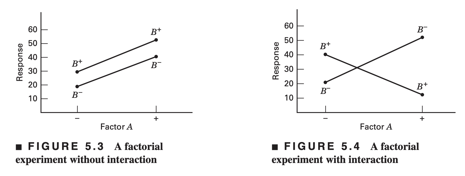
These ideas may be illustrated graphically. Figure 5.3 plots the response data in Figure 5.1 against factor $A$ for both levels of factor $B$.
- Note that the $B-$ and $B+$ lines are approximately parallel, indicating a lack of interaction between factors $A$ and $B$.
Similarly, Figure 5.4 plots the response data in Figure 5.2. Here we see that the $B−$ and $B+$ lines are not parallel.
- This indicates an interaction between factors $A$ and $B$.

There is another way to illustrate the concept of interaction. Suppose that both of our design factors are quantitative (such as temperature, pressure, time).
Then a regression model representation of the two-factor factorial experiment could be written as \[y=\beta_0+\beta_1 x_1 + \beta_2 x_2 + \beta_{12} x_1x_2+\epsilon\]
- where $y$ is the response and the variables x1 and x2 are defined on a coded scale from −1 to +1 (the low and high levels of $A$ and $B$).

The parameter estimates in this regression model turn out to be related to the effect estimates.
For the experiment shown in Figure 5.1 we found the main effects of A and $B$ to be A = 21 and $B$ = 11.
The least square estimates of $\beta_1$ and $\beta_2$are one-half the value of the corresponding main effect (more on this later)

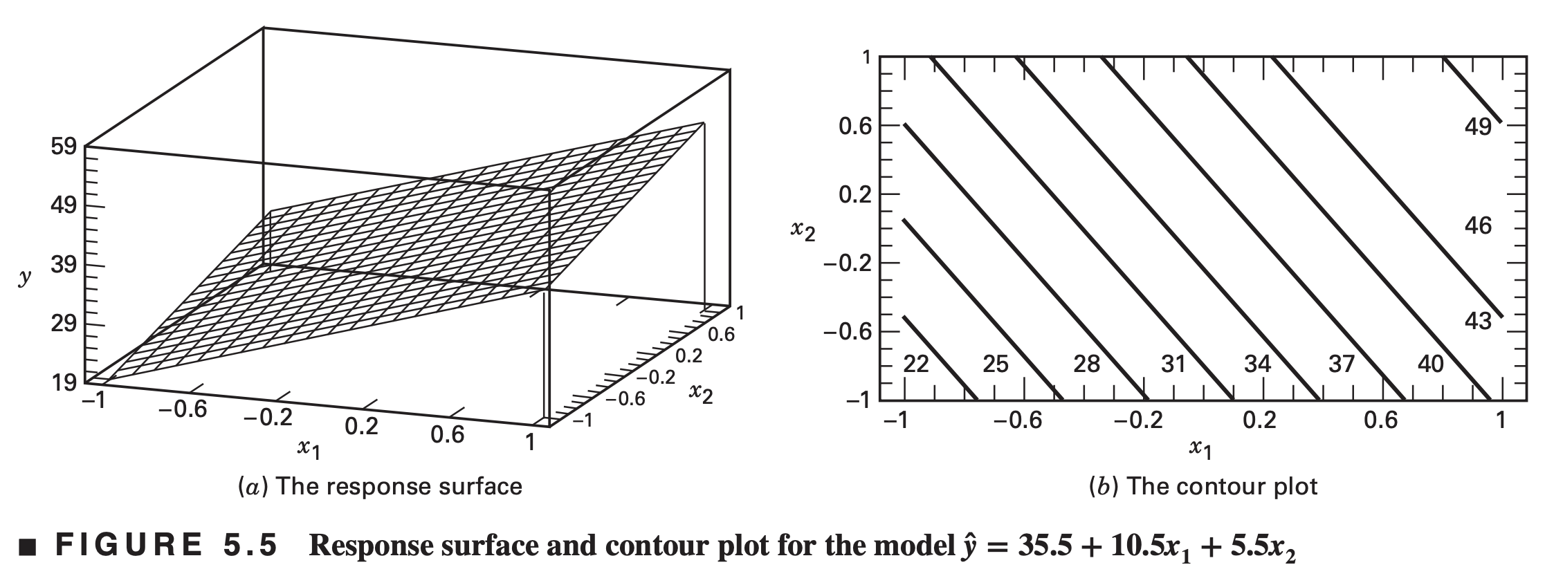
\[ \hat{y} = 35.5 + 10.5 x_1 + 5.5 x_2 + 0.5 x_1 x_2 \equiv 35.5 + 10.5 x_1 + 5.5 x_2 \]

Now suppose that the interaction contribution to this experiment was not negligible
Figure 5.6 presents the response surface and contour plot for the model \[\hat{y} = 35.5 + 10.5 x_1 + 5.5 x_2 + 8 x_1 x_2 \]

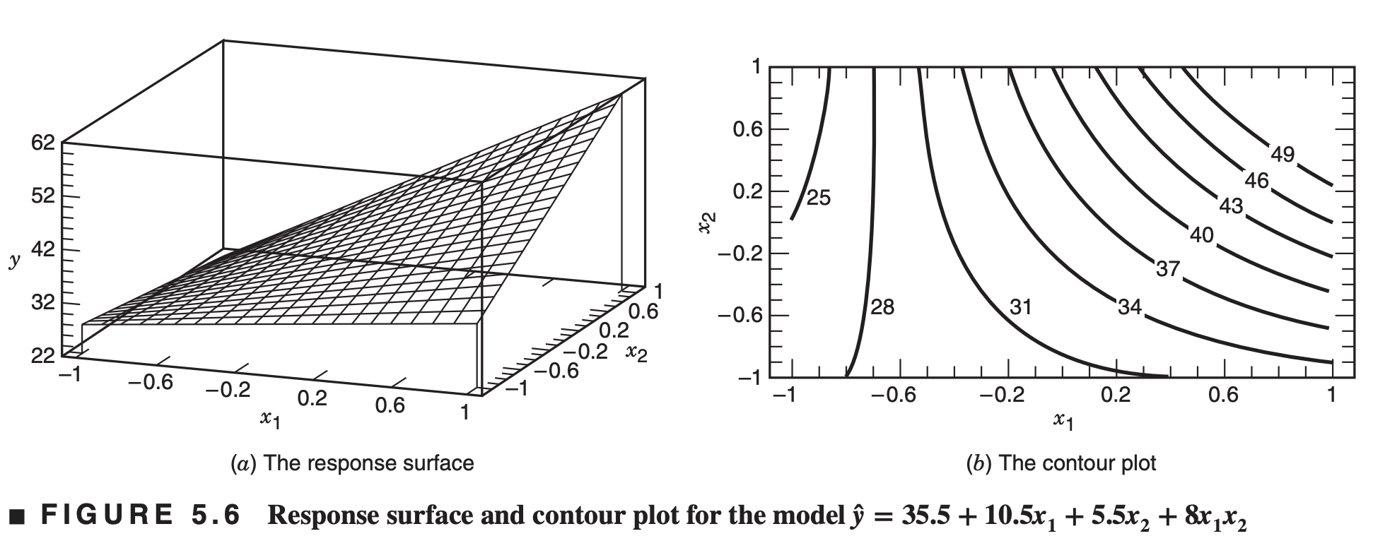
Interaction is a form of curvature in the underlying response surface model for the experiment

5.2 The advantage of factorials

Two factors both at two levels: $A^{+}, A^{-}, B^{+}, B^{-}$
Two possible designs

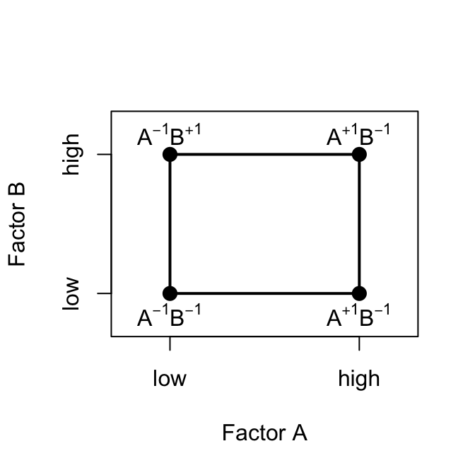
One-factor-at-a-time design

Because experimental error is present, it is desirable to take two observations, say, at each treatment combination and estimate the effects of the factors using average responses.
Thus, a total of six observations are required.
Effects of factors $A$ and $B$ can be obtained, but interaction cannot be calculated

Two-factor factorial design

Using just four observations, two estimates of the $A$ effect can be made. Similarly, two estimates of the $B$ effect can be made.
These two estimates of each main effect could be averaged to produce average main effects that are just as precise as those from the single-factor experiment
Main effects of $A$ and $B$ and their interaction can be calculated

Factorial designs are more efficient than one-factor-at-a-time experiments.
- For this example, the relative efficiency of the factorial design to the one-factor-at-a-time experiment is (6/4) = 1.5.
- Generally, this relative efficiency will increase as the number of factors increases.
A factorial design is necessary when interactions may be present to avoid misleading conclusions.
Factorial designs allow the effects of a factor to be estimated at several levels of the other factors, yielding conclusions that are valid over a range of experimental conditions.

5.3 Two-Factor factorial design

An Example

The simplest types of factorial designs involve only two factors or sets of treatments.
Factor $A$ has $a$ levels and factor $B$ has $b$ levels, so there will be in total $ab$ treatment combinations and each treatment combination is replicated $n$ times

Battery life experiment

An engineer is designing a battery for use in a device that will be subjected to some extreme variations in temperature. The only design parameter that he can select at this point is the plate material for the battery, and he has three possible choices. When the device is manufactured and is shipped to the field, the engineer has no control over the temperature extremes that the device will encounter, and he knows from experience that temperature will probably affect the effective battery life. However, temperature can be controlled in the product development laboratory for the purposes of a test.

The engineer decides to test all three plate materials at three temperature levels - 15, 70, and 125°F - because these temperature levels are consistent with the product end-use environment.
Four batteries are tested at each combination of plate material and temperature, and all 36 tests are run in random order.
The experiment and the resulting observed battery design experiment are given below

$A \rightarrow$ Material type; $B\rightarrow$ Temperature (a quantitative variable)

Important questions:

What effects do material type and temperature have on the life of the battery?
Is there a choice of material that would give uniformly long life regardless of temperature?

General notations

$y_{ijk}$ denotes the observed response when factor $A$ is at the $i^\text{th}$ level $(i=1,2, \ldots, a)$ and factor $B$ is at the $j^\text{th}$ level $(j=1,2, \ldots, b)$ for the $k^\text{th}$ replicate $(k=1,2, \ldots, n)$.
The order in which the $abn$ observations are taken is selected at random so that this design is a completely randomized design.
Data layout

Modelling data

The observations in a factorial experiment can be described by a model. There are several ways to write the model for a factorial experiment.
The means model \[\begin{align*} y_{ijk} = \mu_{ij} + \epsilon_{ijk}\;\;\; \left\{\begin{array}{l} i=1, \ldots, a \\ j=1, \ldots, b \\ k=1, \ldots, n\end{array}\right. \end{align*}\] where $\mu_{ij}$ is the mean corresponding to the treatment combination $i^\text{th}$ level of factor $A$ and $j^\text{th}$ level of factor $B$, and $\epsilon_{ijk}$ is the random error term.
The treatment model (or effects model) \[ y_{ijk} = \mu + \tau_{i} + \beta_j + (\tau\beta)_{ij} +\epsilon_{ijk} \tag{5.1}\] where $\mu$ is the overall mean, $\tau_i$ is the effect of the $i^\text{th}$ level of factor $A$, $\beta_j$ is the effect of the $j^\text{th}$ level of factor $B$, $(\tau\beta)_{ij}$ is the interaction between $\tau_i$ and $\beta_j$.

We could also use a regression model as in Section 5.1 (particularly useful when one or more of the factors in the experiment are quantitative).
Throughout most of this chapter we will use the effects model (Equation 5.1) with an illustration of the regression model in Section 5.5.

In the two-factor factorial, both row and column factors (or treatments), $A$ and $B$, are of equal interest.
Specifically, we are interested in testing hypotheses about the equality of row treatment effects, say \[\begin{align*} &H_{0}: \tau_{1}=\tau_{2}=\cdots=\tau_{a}=0 \\ &H_{1}: \text{at least one } \tau_{i} \neq 0 \end{align*}\]
and the equality of column treatment effects, say \[\begin{align*} &H_{0}: \beta_{1}=\beta_{2}=\cdots=\beta_{b}=0 \\ &H_{1}: \text {at least one } \beta_{j} \neq 0 \end{align*}\]
We are also interested in determining whether row and column treatments interact: \[\begin{align*} &H_{0}:(\tau \beta)_{i j}=0 \text { for all } i, j \\ &H_{1}: \text {at least one }(\tau \beta)_{i j} \neq 0 \end{align*}\]

Statistical analysis of the fixed effects model

Notations

\[\begin{align*} y_{i\cdot\cdot}&=\sum_{j=1}^b \sum_{k=1}^n y_{ijk} & \bar{y}_{i\cdot\cdot}&= \frac{y_{i\cdot\cdot}}{bn} \;\;\; i=1,\ldots, a\\ y_{\cdot j\cdot}&=\sum_{i=1}^a \sum_{k=1}^n y_{ijk} & \bar{y}_{\cdot j\cdot}&= \frac{y_{\cdot j\cdot}}{an}\;\;\; j=1,\ldots, b \\ y_{ij\cdot}&= \sum_{k=1}^n y_{ijk} & \bar{y}_{ij\cdot}&= \frac{y_{ij\cdot}}{n}\;\; \left. \begin{array}{l} i=1,\ldots, a \\ j=1,\ldots, b\end{array}\right. \\ y_{\cdot\cdot\cdot} &= \sum_{i=1}^a \sum_{j=1}^b \sum_{k=1}^n y_{ijk} & \bar{y}_{\cdot\cdot\cdot} &= \frac{y_{\cdot\cdot\cdot}}{abn} \end{align*}\]

Decomposing total variation

Total corrected sum of squares can be expressed as \[ SS_T = \sum_{i,j,k} (y_{ijk}- \bar{y}_{\cdot\cdot\cdot})^2 = SS_A + SS_B + SS_{AB} + SS_E, \tag{5.2}\] where \[\begin{align*} SS_A &= bn\sum_{i} (\bar{y}_{i\cdot\cdot} - \bar{y}_{\cdot\cdot\cdot})^2 \;\;\;\;\;\; SS_B = an\sum_{j} (\bar{y}_{\cdot j\cdot} - \bar{y}_{\cdot\cdot\cdot})^2\\ SS_{AB} &= n\sum_{i, j} (\bar{y}_{ij\cdot} - \bar{y}_{i\cdot\cdot} - \bar{y}_{\cdot j\cdot} + \bar{y}_{\cdot\cdot\cdot})^2\\ SS_E &= \sum_{i, j, k} (y_{ijk} - \bar{y}_{ij\cdot})^2 \end{align*}\]

Equation 5.2 is the fundamental ANOVA equation for the two-factor factorial

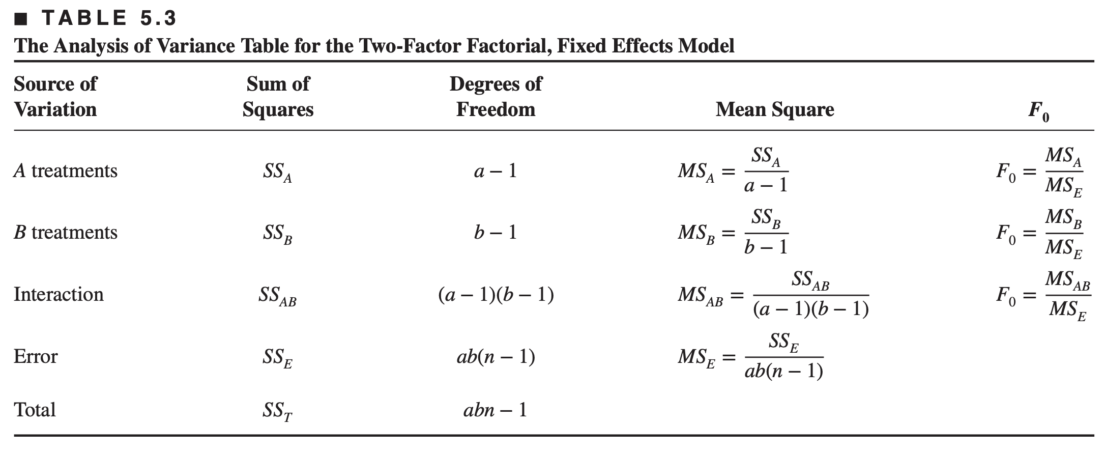
The number of degrees of freedom associated with each sum of squares

\[ \begin{array}{cc} \hline \text{Effect} & \text{Degrees of freedom} \\ \hline A & a-1 \\ B & b-1 \\ A B & (a-1)(b-1) \\ \text{Error} & a b(n-1) \\ \hline \text{Total} & a b n-1 \\ \hline \end{array} \]

Each sum of squares divided by its degrees of freedom is a mean square, e.g. \[ M S_{A}=\frac{S S_{A}}{a-1} \]

Expected value of the mean squares

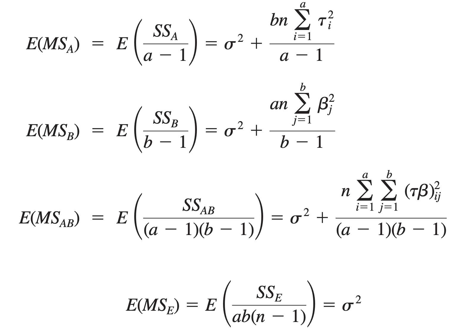
Under the null hypotheses of no treatment effects and no interaction, the $M S_{A}, M S_{B}$, $M S_{A B}$, $MS_E$ all estimate $\sigma^{2}$. If there is significant treatment effect then corresponding mean squares will be larger than $M S_{E}$

Cochran’s theorem

Let $Z_i$ be $\operatorname{NID}(0,1)$ for $i=1,2, \ldots, \nu$ and \[ \sum_{i=1}^\nu Z_i^2=Q_1+Q_2+\cdots+Q_s \] where $s \leq v$, and $Q_i$ has $v_i$ degrees of freedom $(i=1,2, \ldots, s)$. Then $Q_1, Q_2, \ldots, Q_s$ are independent chi-square random variables with $v_1, v_2, \ldots, v_s$ degrees of freedom, respectively, if and only if \[ \nu=\nu_1+\nu_2+\cdots+\nu_s \]

Distributions of sum of squares

For the observed response $y_{ijk}$, $i=1,\ldots, a$, $j=1,\ldots, b$, and $k=1,\ldots, n$, we can decompose the total sum of squares as \[\begin{align*} SS_T &\;\; = \;\; \; SS_A \;\;+\;\; SS_B \;\;+\;\;\;\; SS_{AB}\; \;\;\;\;+\;\;\;\;\; SS_E\\ {\color{blue} (abn-1)} & \;\;\;\;\;\;\; {\color{blue} a-1}\;\;\;\;\;\;\; {\color{blue} b-1} \;\;\;\;\; {\color{blue} (a-1)(b-1)} \;\;\;{\color{blue} ab(n-1)} \end{align*}\]

If $SS_A$, $SS_B$, $SS_{AB}$, and $SS_{E}$ are independent, then using Cochran’s theorem we can write \[ SS_A\sim \chi^2_{(a-1)}, \;\; SS_B\sim\chi^2_{(b-1)}, \;\; SS_{AB}\sim\chi^2_{(a-1)(b-1)},\;\; SS_E\sim\chi^2_{(ab(n-1))} \] since \[ (n-1) = (a-1) + (b-1) + (a-1)(b-1) + ab(n-1) \]

Since $SS_A\sim\chi^2_{(a-1)}$ and $SS_E\sim\chi^2_{(b-1)}$, and $SS_A$ and $SS_E$ are independent, then \[ F_A = \frac{SS_A/(a-1)}{SS_E/(ab(n-1))} = \frac{MS_A}{MS_E} \sim F_{a-1, ab(n-1)}\;\;\; \text{under $H_0$} \]
Similarly, \[\begin{align*} F_B &= \frac{SS_B/(b-1)}{SS_E/(ab(n-1))} = \frac{MS_B}{MS_E} \sim F_{b-1, ab(n-1)}\;\;\; \text{under $H_0$} \\~\\ F_{AB} &= \frac{SS_{AB}/(a-1)(b-1)}{SS_E/(ab(n-1))} = \frac{MS_{AB}}{MS_E} \sim F_{(a-1)(b-1), ab(n-1)}\;\;\; \text{under $H_0$} \end{align*}\]

Analysis of variance table

Manual computing formulas for sum of squares \[\begin{align*} SS_T&=\sum_i\sum_j\sum_k(y_{ijk}-\bar{y}_{\cdot\cdot\cdot})^2=\sum_i\sum_j\sum_ky_{ijk}^2-\frac{{y}_{\cdot\cdot\cdot}^2}{abn} \\ SS_A & = bn\sum_i(\bar{y}_{i\cdot\cdot} - \bar{y}_{\cdot\cdot\cdot})^2 = \frac{1}{bn}\sum_i y_{i\cdot\cdot}^2-\frac{{y}_{\cdot\cdot\cdot}^2}{abn} \\ SS_{B} & = an\sum_j(\bar{y}_{\cdot j\cdot} - \bar{y}_{\cdot\cdot\cdot})^2 = \frac{1}{an}\sum_j y_{\cdot j\cdot}^2-\frac{{y}_{\cdot\cdot\cdot}^2}{abn} \end{align*}\]

Manual computing formulas for sum of squares \[\begin{align*} SS_{AB} &= n\sum_i\sum_j(\bar{y}_{ij\cdot} -\bar{y}_{i\cdot\cdot} - \bar{y}_{\cdot j\cdot} + \bar{y}_{\cdot\cdot\cdot})^2\\ &=n\sum_i\sum_j(\bar{y}_{ij\cdot} - \bar{y}_{\cdot\cdot\cdot})^2 - SS_A - SS_B \;\; ({\color{red} how?})\\ &=SS_{\text{subtotals}} - SS_A - SS_B, \end{align*}\] where \[ SS_{\text{subtotals}} = n\sum_i\sum_j(\bar{y}_{ij\cdot} - \bar{y}_{\cdot\cdot\cdot})^2 = \frac{1}{n} \sum_i\sum_j {y}_{ij\cdot}^2 - \frac{y_{\cdot\cdot\cdot}^2}{abn} \] Then \[\begin{align*} SS_E &= SS_T - SS_{AB} - SS_A - SS_B \\ \text{\color{red} or} & \nonumber \\ SS_E &= SS_T - SS_{subtotals} \end{align*}\]

The battery design experiment

Let $y_{ijk}$ denote the observed lifetime of the battery corresponding to the $k^{\text{th}}$ replication of the treatment combination $i^{\text{th}}$ material type (treatment A) and $j^{\text{th}}$ temperature (treatment B) $(i=1,2,3;\, j=1,2,3;\; k=1,\ldots, 4)$.
Consider the effects model \[ {\color{blue} y_{ijk} = \mu + \tau_i + \beta_j + (\tau\beta)_{ij} + \epsilon_{ijk},} \] where $\mu$ is the overall mean, $\tau_i$ and $\beta_j$ are the effects of the $i^\text{th}$ level of factor $A$ and $j^\text{th}$ level of factor $B$, $(\tau\beta)_{ij}$ is the interction between the $i^\text{th}$ level of factor $A$ and $j^\text{th}$ level of factor $B$.
Random error term $\epsilon_{ijk}$ is assumed to be normally distributed with mean $0$ and a constant variance $\sigma^2$.

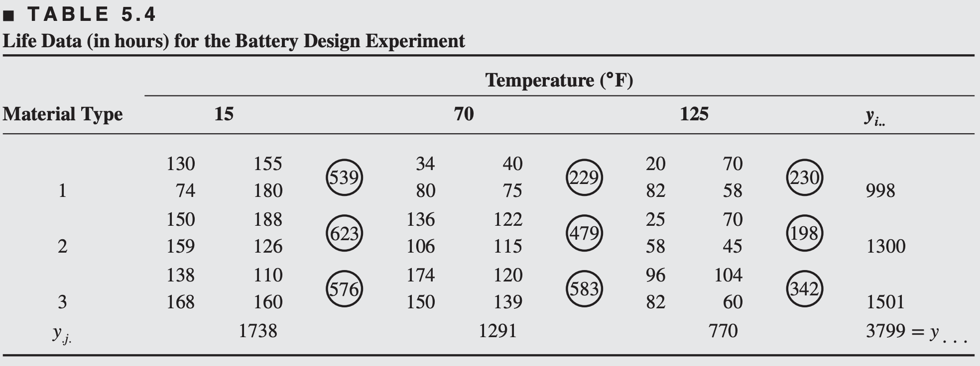
\[\begin{align*} SS_T &= \sum_i\sum_j\sum_j y_{ijk}^2 - \frac{{y}_{\cdot\cdot\cdot}^2}{abn} \\ &= (130)^2 + \cdots + (60)^2 - \frac{(3799)^2}{36}=77646.97 \end{align*}\]

\[\begin{align*} SS_A &= \frac{1}{bn} \sum_i y_{i\cdot\cdot}^2 - \frac{{y}_{\cdot\cdot\cdot}^2}{abn} \\ &= \frac{1}{(3)(4)}\{(998)^2 + (1300)^2 + (1501)^2\} - \frac{(3799)^2}{36}=10683.72 \end{align*}\]

\[\begin{align*} SS_B &= \frac{1}{an} \sum_j y_{\cdot j\cdot}^2 - \frac{{y}_{\cdot\cdot\cdot}^2}{abn} \\ &= \frac{1}{(3)(4)} \{(1738)^2 + (1291)^2 + (770)^2\} - \frac{(3799)^2}{36}=39118.72 \end{align*}\]

\[\begin{align*} SS_{\text{Subtotals}} &= \frac{1}{n} \sum_i\sum_j y_{ij\cdot}^2 - \frac{{y}_{\cdot\cdot\cdot}^2}{abn} \\ &= \frac{1}{4} \{(539)^2 + \cdots + (342)^2\} - \frac{(3799)^2}{36}=49515373 \end{align*}\]

\[\begin{align*} SS_T &= {\color{blue} 77,646.97} \\ SS_A &= {\color{blue} 10,683.72}\\ SS_{B} &={\color{blue} 39118.72}\\ SS_{AB} &= SS_{\text{subtotals}}- SS_A - SS_B \\ &= 49515373 - 10683.72 - 39118.72\\ &= {\color{blue} 9,613.78}\\ SS_E &= SS_T - SS_A - SS_B - SS_{AB} \\ &= 77646.97-10683.72-39118.72-9613.78\\ &={\color{blue} 18,230.78} \end{align*}\]

The battery design experiment (anova table)

There is a significant interaction between material type and temperature
Main effects of material type and temperature are also significant

The battery design experiment (interpreting results)

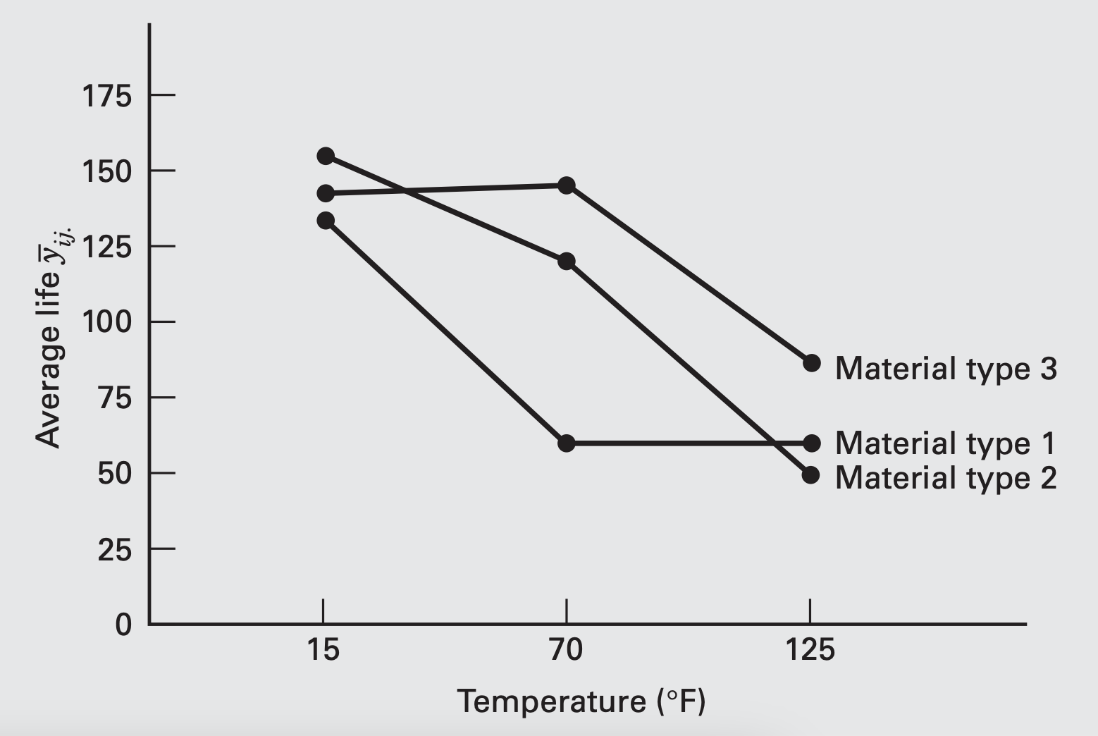
The significant interaction is indicated by the lack of parallelism of the lines
In general, longer life is attained at the low temperature, regardless of material type.
Changing from low to intermediate temperature, battery life with material type 3 increases, whereas it decreases for types 1 and 2.
From intermediate to high temperature, battery life decreases for material types 2 and 3, and is essentially unchanged for type 1.
Material type 3 seems to give the best result if we want less loss of effective life as the temperature changes.

The battery design experiment (multiple comparisons)

One of the goals of the experiment is to identify the best treatment combination. In two-factor factorial experiment, significance of interaction plays an important role in selecting the best treatment combination.

When interaction is not significant, multiple comparison methods can be used to identify the best level for each factor separately.
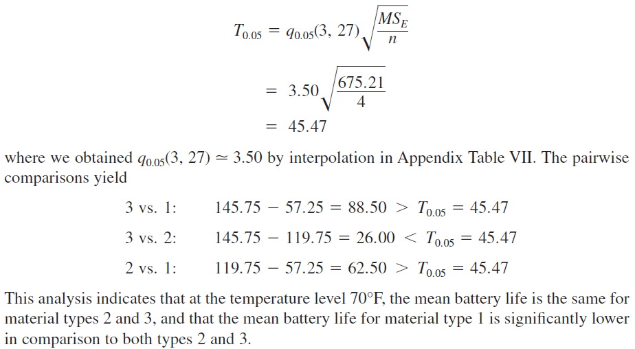
When interaction is significant, the best level of one factor need to be identified at each level of the other factor. e.g. comparisons between the means of factor $A$ can be obtained for a specific level of factor $B$ applying Tukey’s test.

Suppose we are interested in detecting differences among the means of the three material types.
Because interaction is significant, we make this comparison at just one level of temperature, say level 2 (70°F)
The three material type averages at $70^{\circ} \mathrm{F}$ arranged in ascending order are \[ \begin{array}{ll} \bar{y}_{12 .}=57.25 & (\text { material type } 1) \\ \bar{y}_{22 .}=119.75 & (\text { material type 2) } \\ \bar{y}_{32 .}=145.75 & (\text { material type } 3) \end{array} \]

Model adequacy checking

Before making the conclusions from the analysis of variance, the adequacy of the underlying model should be checked using residual analysis (e.g. checking normality, independence, constant variance, etc.).
The residuals for the two-factor factorial model \[\begin{align*} e_{ijk} &= y_{ijk} - \hat{y}_{ijk} \\ & = y_{ijk} - \bar{y}_{ij\cdot} \end{align*}\]
Different tools of residual analysis:
- q-q normal plot of residuals
- Plot of residuals against fitted values
- Plot of residuals against different factors separately

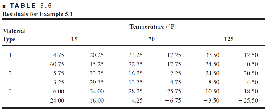
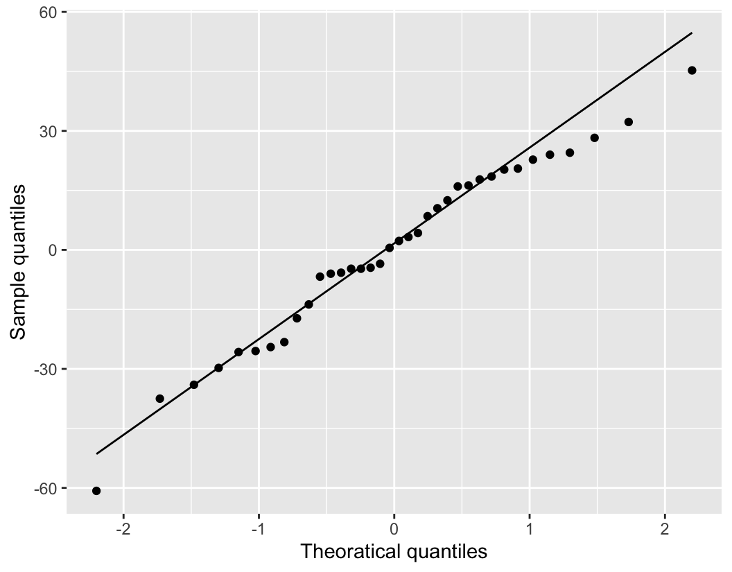
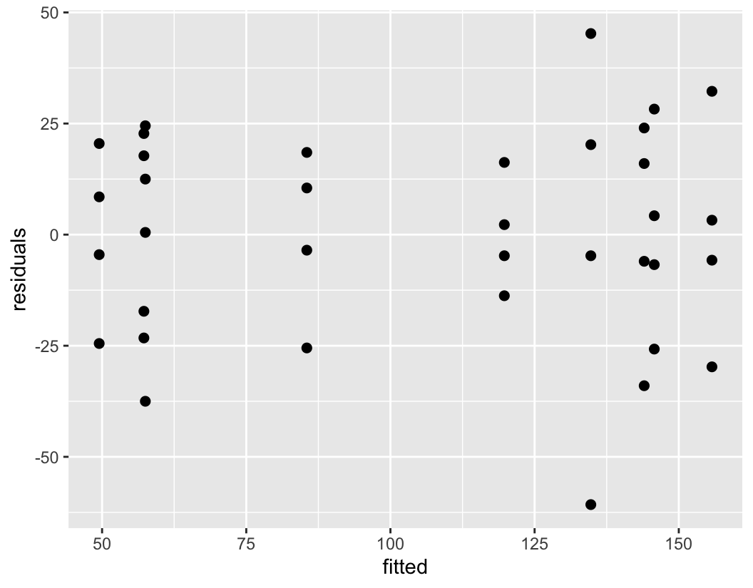
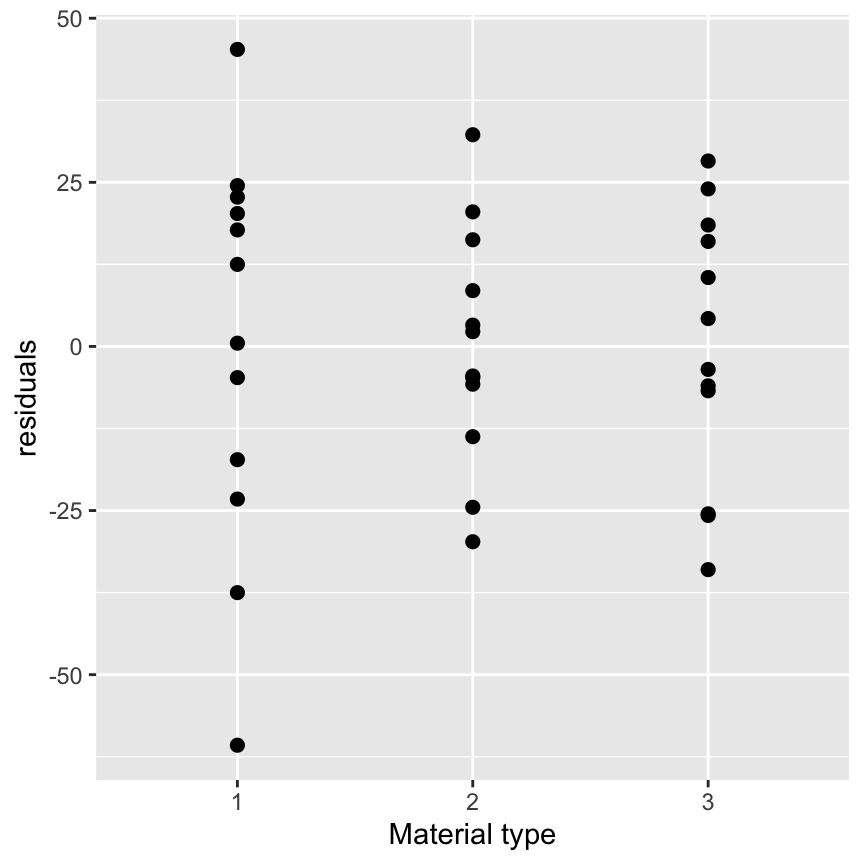
Estimating model parameters

The effects model for two-factor factorial is \[ y_{ijk} = \mu + \tau_i + \beta_j + (\tau\beta)_{ij} + \epsilon_{ijk}, \tag{5.3}\] where $\mu$, $\tau_i$, $\beta_j$, and $(\tau\beta)_{ij}$ are parameters of interest, and random error term is assumed to be normally distributed, i.e. \[\epsilon_{ijk}\sim \mathcal{N}(0, \sigma^2)\;\;\Rightarrow\;\; y_{ijk}\sim\mathcal{N}(\mu_{ij}, \sigma^2)\]

They may be estimated by least squares. Because the model has $1 + a + b + ab$ parameters to be estimated, and there $1 + a + b + ab$ normal equations.

Using the method of Section 3.9, we find that it is not difficult to show that the normal equations are

The effects model (Equation 5.3) is an overparameterized model.
Notice that the $a$ equations in Equation 5.14b sum to Equation 5.14a and that the $b$ equations of Equation 5.14c sum to Equation 5.14a.
Also summing Equation 5.14d over $j$ for a particular $i$ will give Equation 5.14b, and summing Equation 5.14d over $i$ for a particular $j$ will give Equation 5.14c.
Therefore, there are $a + b + 1$ linear dependencies in this system of equations, and no unique solution will exist.
In order to obtain a solution, we impose the constraints

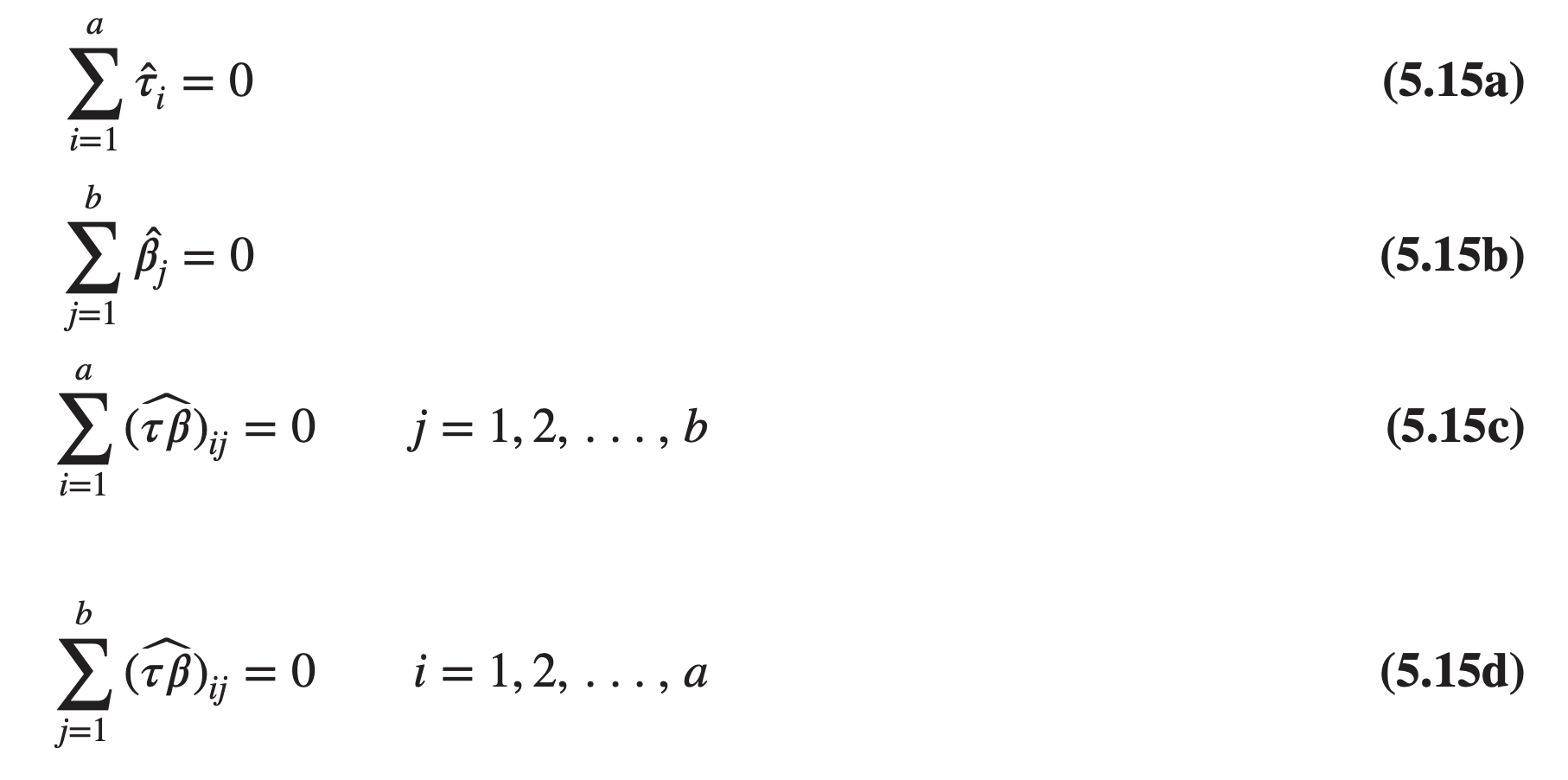
Equations 5.15a and 5.15b constitute two constraints, whereas Equations 5.15c and 5.15d form $a + b − 1$ independent constraints. Therefore, we have $a + b + 1$ total constraints, the number needed.

Applying these constraints, the normal equations (Equations 5.14) simplify considerably, and we obtain the solution

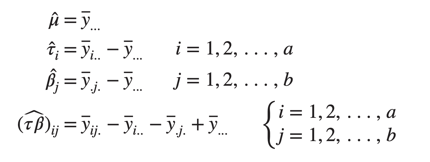
The MLE

The log-likelihood function \[\begin{align*} l(\boldsymbol{\theta}) &= \sum_i\sum_j\sum_k \Big\{ -\frac{\operatorname{log}{\sigma^2}}{2} -\frac{1}{2\sigma^2}\Big(y_{ijk} - \mu_{ij}\big)^2 + constant\Big\}, \end{align*}\] where $\boldsymbol{\theta}=\{\mu, \, \tau_i, \, \beta_j, \, (\tau\beta)_{ij}\}$ is the vector of parameters of order $1 + a + b + ab$.

\[ SSE=\sum_{i=1}^a \sum_{j=1}^b \sum_{k=1}^n \epsilon_{i j k}^2=\sum_{i=1}^a \sum_{j=1}^b \sum_{k=1}^n\left(y_{i j k}-\mu_{ij}\right)^2. \]

Here \[\hat{\boldsymbol{\theta}}_{MLE} = arg\,max \,\, l(\boldsymbol{\theta}) \] \[\hat{\boldsymbol{\theta}}_{LSE} = arg\,min \,\, SSE=arg\,max \,\, l(\boldsymbol{\theta})\]
Therefore, the solutions obtained (through LSE) are also MLE.

Choice of sample size

In any experimental design problem, a critical decision is the choice of sample size — that is, determining the number of replicates to run.
Generally, if the experimenter is interested in detecting small effects, more replicates are required than if the experimenter is interested in detecting large effects.

OC (Operating Characteristic) curve

An operating characteristic (OC) curve is a plot of the type II error probability $(\beta)$ of a statistical test for a particular sample size versus a parameter $\Phi$ that reflects the extent to which the null hypothesis is false.
These curves can be used to guide the experimenter in selecting the number of replicates so that the design will be sensitive to important potential differences in the treatments.
The operating characteristic curves in Appendix Chart V (Montgomery book) can be used to assist the experimenter in determining an appropriate sample size (number of replicates, $n$) for a two-factor factorial design.
Curves are available for $\alpha=0.05$ and $\alpha=0.01$ and a range of degrees of freedom for numerator and denominator.

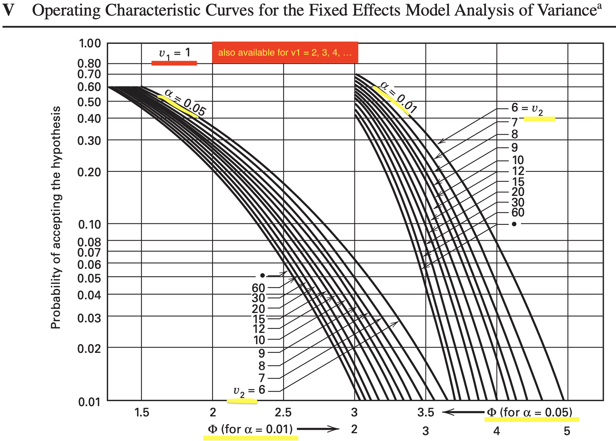
OC curve for two-factor factorial design

OC Curve parameters for chart V of the Appendix for the two-factor factorial, fixed effects model

\[ \begin{array}{lccc} \hline \text{Factor} & \Phi^2 & \text{Numerator DF} & \text{Denominator DF} \\ \hline A & \frac{b n \sum_{i=1}^a \tau_i^2}{a \sigma^2} & a-1 & a b(n-1) \\ B & \frac{a n \sum_{j=1}^b \beta_j^2}{b \sigma^2} & b-1 & a b(n-1) \\ A B & \frac{n \sum_{i=1}^a \sum_{j=1}^b(\tau \beta)_{i j}^2 }{\sigma^2 [(a-1)(b-1) +1]} & (a-1)(b-1)& a b(n-1) \\ \hline \end{array} \]

For two-factor factorial design, the appropriate value of the parameter $\Phi$ and the numerator and denominator degrees of freedom are shown in the table.

To determine $\Phi$, we need to know the actual values of the treatment means on which the sample size decision should be based. If we know that, we can use the formulas of the table and proceed as the one-factor design. But a set of actual treatment means is not available most of the time.
An alternate approach is to select a sample size such that if the difference between any two treatment means exceeds a specified value, the null hypothesis should be rejected.

For example, if the difference in any two row (Factor $A$) means is $D$, then the minimum value of $\Phi^2$ is \[ \Phi^2=\frac{n b D^2}{2 a \sigma^2} \]
If the difference in any two column (Factor $B$) means is $D$, then the minimum value of $\Phi^2$ is \[ \Phi^2=\frac{n a D^2}{2 b \sigma^2} \]
Finally, the minimum value of $\Phi^2$ corresponding to a difference of $D$ between any two interaction effects is \[ \Phi^2=\frac{n D^2}{2 \sigma^2[(a-1)(b-1)+1]}. \]

OC curve(Battery design experiment)

To illustrate the use of these equations, consider the battery design experiment.
Suppose that before running the experiment we decide that the null hypothesis should be rejected with a high probability if the difference in mean battery life between any two temperatures is as great as 40 hours.
Thus a difference of $D=40$ has engineering significance, and if we assume that the standard deviation of battery life is approximately 25 , then the corresponding equation gives \[\begin{align*} \Phi^2 &=\frac{n a D^2}{2 b \sigma^2} \\ &=\frac{n(3)(40)^2}{2(3)(25)^2} \\ &=1.28 n \end{align*}\]

as the minimum value of $\Phi$.

Assuming that $\alpha=0.05$, we can now use Appendix Table V to construct the following display:

\[ \begin{array}{cccccc} \hline & & & {\nu}_{\mathbf{1}}= \text{Numerator} & {\nu}_2= \text{Error} & \\ {n}& {\Phi}^{\mathbf{2}} & {\Phi} & \text{Degrees of Freedom} & \text{Degrees of Freedom} & {\beta} \\ \hline 2 & 2.56 & 1.60 & 2 & 9 & 0.45 \\ 3 & 3.84 & 1.96 & 2 & 18 & 0.18 \\ 4 & 5.12 & 2.26 & 2 & 27 & 0.06 \\ \hline \end{array} \]

Note that $n=4$ replicates give a $\beta$ risk of about 0.06, or approximately a 94 percent chance of rejecting the null hypothesis if the difference in mean battery life at any two temperature levels is as large as 40 hours.
Thus, we conclude that four replicates are enough to provide the desired sensitivity as long as our estimate of the standard deviation of battery life is not seriously in error.
If in doubt, the experimenter could repeat the above procedure with other values of $\sigma$ to determine the effect of mis-estimating this parameter on the sensitivity of the design.

Assumption of no interaction in a two-factor model

Occasionally, an experimenter feels that a two-factor model without interaction is appropriate, say \[ y_{ijk} = \mu + \tau_{i} + \beta_j +\epsilon_{ijk} \left\{\begin{array}{l}i=1,2, \ldots, a \\ j=1,2, \ldots, b \\ k=1,2, \ldots, n\end{array}\right.\]

The statistical analysis of a two-factor factorial model without interaction is straightforward. The following table presents the analysis of the battery design experiment, assuming no interaction.

\[ \begin{array}{lccrr} \hline \text{Source of} & \text{Sum} & \text{Degrees} & \text{Mean} & \\ \text{Variation} & \text{of Squares} & \text{of Freedom} & \text{Square} & {F}_{{0}} \\ \hline \text{Material types} & 10,683.72 & 2 & 5,341.86 & 5.95 \\ \text{Temperature} & 39,118.72 & 2 & 19,559.36 & 21.78 \\ \text{Error} & 27,844.52 & 31 & 898.21 & \\ \text{Total} & 77,646.96 & 35 & & \\ \hline \end{array} \]

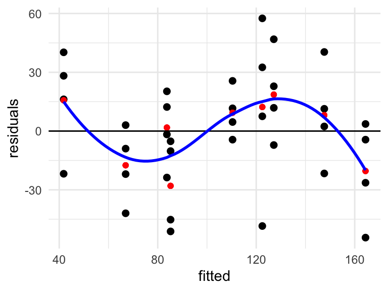
As noted previously, both main effects are significant. However, as soon as a residual analysis is performed for these data, it becomes clear that the no-interaction model is inadequate.

For the two-factor model without interaction, the fitted values are $\hat{y}_{i j k}=\bar{y}_{i . .}+\bar{y}_{j .}-\bar{y}_{. . .}$. A plot of fitted versus residuals is shown below.

One observation per cell

Occasionally, one encounters a two-factor experiment with only a single replicate, that is, only one observation per cell. If there are two factors and only one observation per cell, the effects model is \[ y_{i j}=\mu+\tau_i+\beta_j+(\tau \beta)_{i j}+\epsilon_{i j} \quad\left\{\begin{array}{l} i=1,2, \ldots, a \\ j=1,2, \ldots, b \end{array}\right. \]

The analysis of variance for this situation is shown in Table 5.9, assuming that both factors are fixed.

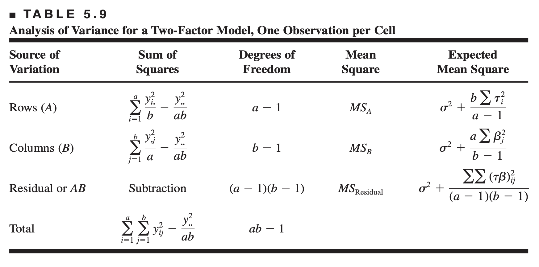
From examining the expected mean squares, we see that the error variance $\sigma^2$ is not estimable; that is, the two-factor interaction effect $(\tau \beta)_{i j}$ and the experimental error cannot be separated in any obvious manner. Consequently, there are no tests on main effects unless the interaction effect is zero. If there is no interaction present, then $(\tau \beta)_{i j}=0$ for all $i$ and $j$, and a plausible model is \[ y_{i j}=\mu+\tau_i+\beta_j+\epsilon_{i j} \quad\left\{\begin{array}{l} i=1,2, \ldots, a \\ j=1,2, \ldots, b \end{array}\right. \] If this later model is appropriate, then the residual mean square in Table 5.9 is an unbiased estimator of $\sigma^2$, and the main effects may be tested by comparing $M S_A$ and $M S_B$ to $M S_{\text {Residual }}$.

5.4 The general factorial design

General factorial design

The two-factor factorial design may be extended to the general case where there are a levels of factor $A$, $b$ levels of factor $B$, $c$ levels of factor $C$, and so on.

In general, there will be $abc \ldots n$ total observations if there are $n$ replicates of the complete experiment.

Note that we must have at least two replicates $(n \ge 2)$ to determine a sum of squares due to error if all possible interactions are included in the model.

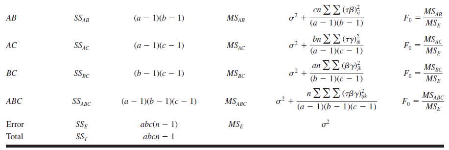
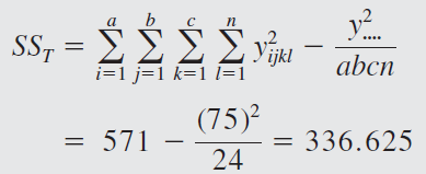
For example, consider the three-factor analysis of variance model: \[y_{i j k l}=\mu+\tau_i+\beta_j+\gamma_k+(\tau \beta)_{i j}+(\tau \gamma)_{i k}+(\beta \gamma)_{j k}+ (\tau \beta \gamma)_{i j k}+\epsilon_{i j k l}\]

$\left\{\begin{array}{l}i=1,2, \ldots, a \\ j=1,2, \ldots, b \\ k=1,2, \ldots, c \\ l=1,2, \ldots, n\end{array}\right.$

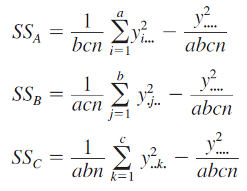
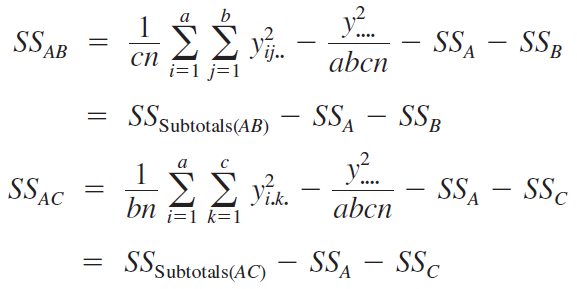
Assuming $A$, $B$, and $C$ are fixed, the ANOVA table is

Soft drink bottling problem

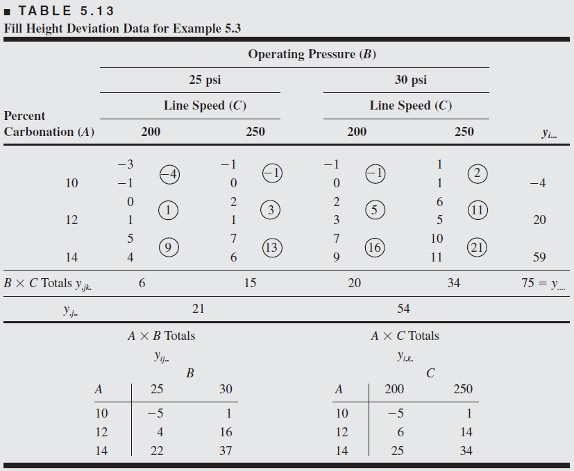
A soft drink bottler is interested in obtaining more uniform fill heights in the bottles produced by his manufacturing process. The filling machine theoretically fills each bottle to the correct target height, but in practice, there is variation around this target, and the bottler would like to understand the sources of this variability better and eventually reduce it.

The process engineer can control three variables during the filling process: the percent carbonation (A), the operating pressure in the filler (B), and the bottles produced per minute or the line speed (C). For purposes of an experiment, the engineer can control carbonation at three levels: 10, 12, and 14 percent. She chooses two levels for pressure (25 and 30 psi) and two levels for line speed (200 and 250 bpm)

The engineer decides to run two replicates of a factorial design in these three factors, with all 24 runs taken in random order. The response variable observed is the average deviation from the target fill height observed in a production run of bottles at each set of conditions. Positive deviations are fill heights above the target, whereas negative deviations are fill heights below the target. The circled numbers are the three-way cell totals $y_{ijk}$.

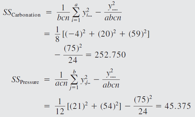
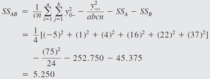
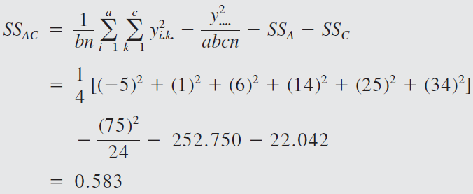
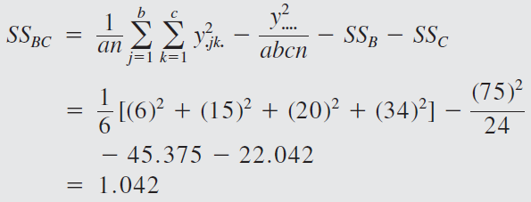
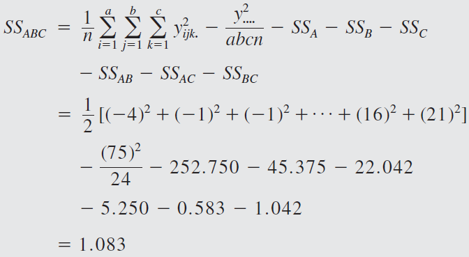
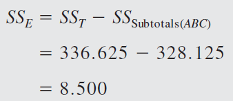
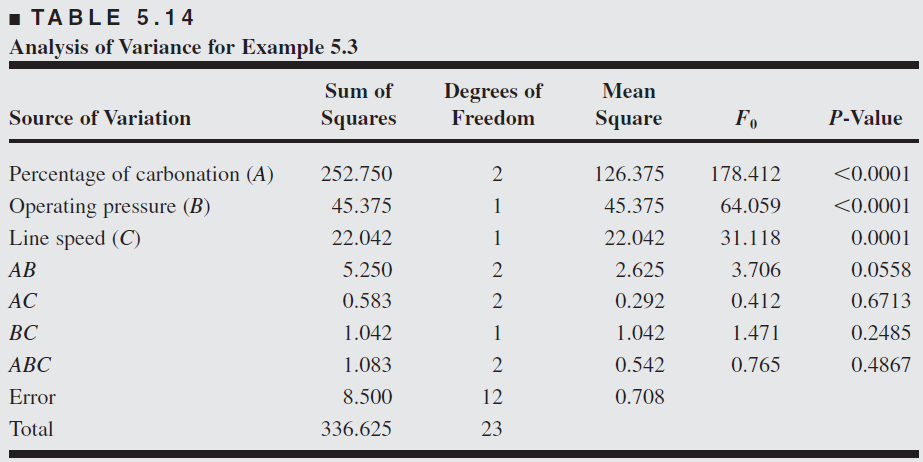
From the ANOVA we see that the percentage of carbonation, operating pressure, and line speed significantly affect the fill volume.

The carbonation pressure interaction $F$ ratio has a $p$-value of 0.0558, indicating some interaction between these factors.

To assist in the practical interpretation of this experiment, the following figure presents plots of the three main effects and the $AB$ (carbonation– pressure) interaction.

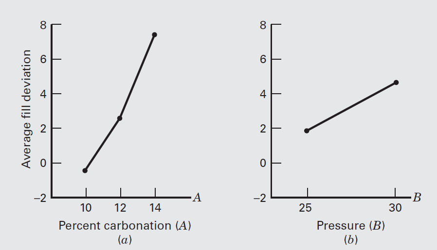
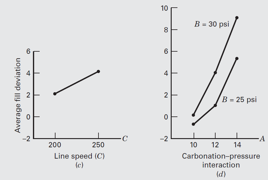
The main effect plots are just graphs of the marginal response averages at the levels of the three factors. Notice that all three variables have positive main effects; that is, increasing the variable moves the average deviation from the fill target upward.

The interaction between carbonation and pressure is fairly small, as shown by the similar shape of the two curves.

5.5 Fitting Response Curves and Surfaces

The ANOVA always treats all of the factors in the experiment as if they were qualitative or categorical. Many experiments involve at least one quantitative factor. It can be useful to fit a response curve to the levels of a quantitative factor so that the experimenter has an equation that relates the response to the factor

This equation might be used for interpolation, that is, for predicting the response at factor levels between those actually used in the experiment. When at least two factors are quantitative, we can fit a response surface for predicting y at various combinations of the design factors. In general, linear regression methods are used to fit these models to the experimental data

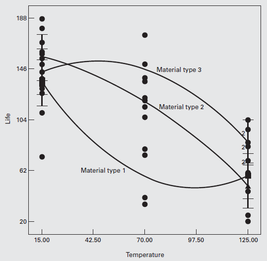
The battery design experiment

Consider the battery life experiment described previously. The factor temperature is quantitative, and the material type is qualitative.

Furthermore, there are three levels of temperature.

Consequently, we can compute a linear and a quadratic temperature effect to study how temperature affects the battery life.

Because material type is a qualitative factor there is an equation for predicted life as a function of temperature for each material type.

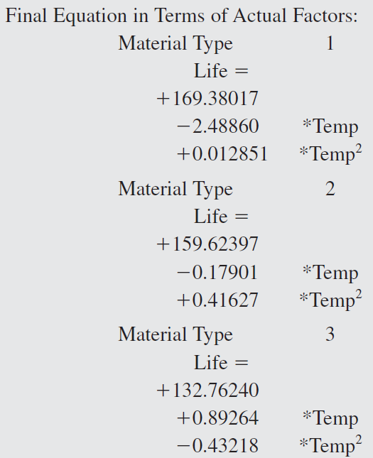
Figure 5.18 shows the response curves generated by these three prediction equations.

5.6 Blocking in a facorial design

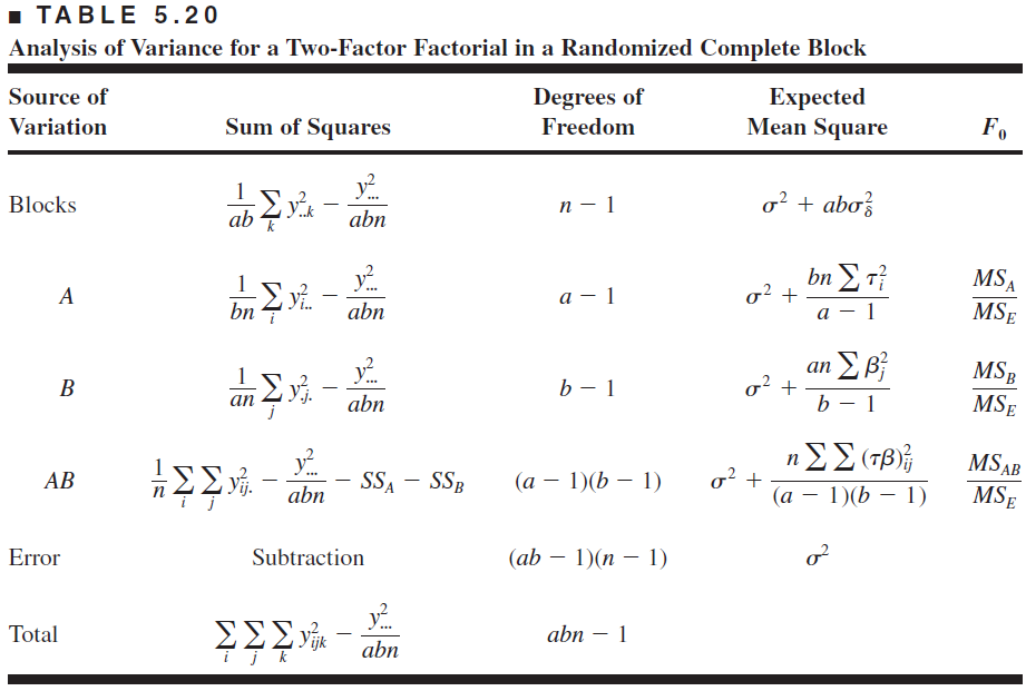
\[ y_{i j k}=\mu+\tau_i+\beta_j+(\tau \beta)_{i j}+\delta_k+\epsilon_{i j k} \quad\left\{\begin{array}{l} i=1,2, \ldots, a \\ j=1,2, \ldots, b \\ k=1,2, \ldots, n \end{array}\right. \] where $\delta_k$ is the effect of the $k$ th block. Of course, within a block the order in which the treatment combinations are run is completely randomized.

Example 5.6

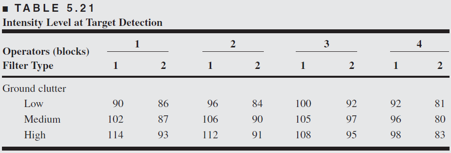
An engineer is studying methods for improving the ability to detect targets on a radar scope. Two factors she considers to be important are the amount of background noise, or ground clutter, on the scope and the type of filter placed over the screen. An experiment is designed using 3 levels of ground clutter and 2 filter types.

Because of operator availability, it is convenient to select an operator and keep him or her at the scope until all the necessary runs have been made. Furthermore, operators differ in their skill and ability to use the scope. Consequently, it seems logical to use the operators as blocks.

Four operators are randomly selected. Once an operator is chosen, the order in which the six treatment combinations are run is randomly determined.

Thus, we have a $3 \times 2$ factorial experiment run in a randomized complete block. The data are shown below

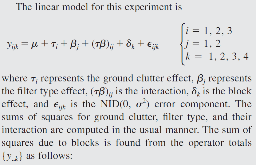
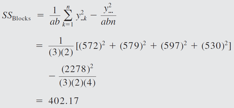
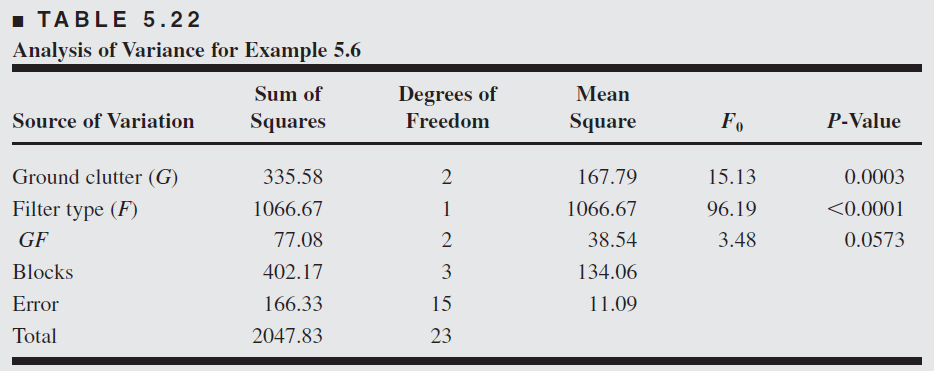
Both ground clutter level and filter type are significant at the 1 percent level, whereas their interaction is significant only at the 10 percent level.

Thus, we conclude that both ground clutter level and the type of scope filter used affect the operator’s ability to detect the target, and there is some evidence of mild interaction between these factors.

Exercise

The following output was obtained from a computer program that performed a two-factor ANOVA on a factorial experiment.

Fill in the blanks in the ANOVA table. You can use bounds on the p-values.
How many levels were used for factor $B$?
How many replicates of the experiment were performed?
What conclusions would you draw about this experiment?

Practice exercises from Montgomery book:

5.41, 5.42, 5.43, 5.44, 5.45, 5.46