Chapter 13

(AST301) Design and Analysis of Experiments II

13 Experiments with Random Factors

13.1 Introduction

Throughout most of this book we have assumed that the factors in an experiment were fixed factors, that is, the levels of the factors used by the experimenter were the specific levels of interest.

The implication of this, of course, is that the statistical inferences made about these factors are confined to the specific levels studied.

That is, if three material types are investigated as in the battery life experiment of Example 5.1, our conclusions are valid only about those specific material types.

---

A variation of this occurs when the factor or factors are quantitative. In these situations, we often use a regression model relating the response to the factors to predict the response over the region spanned by the factor levels used in the experimental design.

Several examples of this were presented in Chapters 5 through 9. In general, with a fixed effect, we say that the inference space of the experiment is the specific set of factor levels investigated.

---

In some experimental situations, the factor levels are chosen at random from a larger population of possible levels, and the experimenter wishes to draw conclusions about the entire population of levels, not just those that were used in the experimental design.

In this situation, the factor is said to be a random factor.

The random effect model was introduced in Chapter 3 for a single-factor experiment, and we used that to introduce the random effects model for the analysis of variance and components of variance.

---

For example: a company has 50 machines that make cardboard cartons for canned goods, and they want to understand the variation in strength of the cartons.

They choose ten machines at random from the 50 and make 40 cartons on each machine, assigning 400 lots of feedstock cardboard at random to the ten chosen machines.

The resulting cartons are tested for strength. This is a completely randomized design, with ten treatments and 400 units.

---

Fixed Effects Model

$$\begin{array}{rl}{y}_{ij}& =\mu +{\tau }_i+{ϵ}_{ij}\\ {ϵ}_{ij}& \sim N(0,{\sigma }^2)\end{array}$$

• $\mu$: overall mean
  
• ${\tau }_i$: fixed effect of treatment $i$
  
• ${ϵ}_{ij}$: random error
  
• ${\tau }_i$ are fixed unknown parameters

Random Effects Model

$$\begin{array}{rl}{y}_{ij}& =\mu +{\tau }_i+{ϵ}_{ij}\\ {\tau }_i& \sim N(0,{\sigma }_{\tau }^2)\\ {ϵ}_{ij}& \sim N(0,{\sigma }^2)\end{array}$$

• $\mu$: overall mean
  
• ${\tau }_i$: random effect of treatment $i$
  
• ${ϵ}_{ij}$: random error
  
• ${\tau }_i$ are random variables

• Notice that we still decompose the model into: Overall mean ($\mu$), Treatment effect (${\tau }_i$), Random error (${ϵ}_{ij}$)

• Why Fixed-Effects Assumptions Don’t Make Sense in Random Effects Model?

---

1. Treatment levels are not fixed but randomly sampled

• In the fixed-effects model, the treatment levels (e.g., different brands, machines, or methods) are specifically chosen and of interest.

• In the random-effects model, these levels are assumed to be a random sample from a larger population of possible treatments.

• Therefore, estimating individual treatment effects (${\tau }_i$) is less meaningful — we care more about the variation among treatments, not their specific values.

---

2. The focus shifts from estimation to generalization

• In fixed-effects, we want to compare specific treatment effects.

• In random-effects, we aim to generalize to the broader population of treatments.

• So, we’re more interested in estimating variance components (like ${\sigma }_{\tau }^2$) to understand how much treatments vary, not just how they differ.

---

3. Inference is about variance components

• In random-effects, variability in treatment levels is treated as another source of random variation.

• This affects how we partition the total variance and how we perform statistical inference (like testing and confidence intervals).

---

In this chapter, we focus on methods for the design and analysis of factorial experiments with random factors.

In Chapter 14, we will present nested and split-plot designs, two situations where random factors are frequently encountered in practice.

Review: Random Effects Model

• Random effects model is defined only for the random factors, e.g. $$y_{ij}=\mu +{\tau }_i+{ϵ}_{ij},i=1,\dots ,a;j=1,\dots ,n$$ where both ${\tau }_i$ and ${ϵ}_{ij}$ are random variables (${\tau }_i$ is not parameter), which are assumed to follow $\mathcal{N}(0,{\sigma }_{\tau }^2)$ and $\mathcal{N}(0,{\sigma }^2)$, respectively.

• ${\tau }_i$ and ${ϵ}_{ij}$ are independent

• Variance structure $$\text{cov}(y_{ij},y_{i^{\prime }{j}^{\prime }})=\{\begin{array}{ll}{\sigma }_{\tau }^2+{\sigma }^2& \text{if}i=i^{\prime },j=j^{\prime }\\ {\sigma }_{\tau }^2& \text{if}i=i^{\prime },j\ne j\\ 0& \text{if}i\ne i^{\prime }\end{array}$$

• ${\sigma }_{\tau }^2$ and ${\sigma }^2$ are known as variance components

---

The parameters of the random effects model are the overall mean $\mu$, the error variance ${\sigma }^2$, and the variance of the treatment effects ${\sigma }_{\tau }^2$; the treatment effects ${\tau }_i$ are random variables, not parameters.

We want to make inferences about these parameters; we are not so interested in making inferences about the ${\tau }_i$ ’s and ${ϵ}_{ij}$ ’s.

Typical inferences would be point estimates or confidence intervals for the variance components, or a test of the null hypothesis that the treatment variance ${\sigma }_{\tau }^2$ is 0

---

• Hypothesis considered for the fixed effects model $$H_0:\text{no difference between treatment levels}$$ is no longer useful for the random effects model

• For random effects model the hypothesis regarding no treatment effects is defined as $$H_0:{\sigma }_{\tau }^2=0vs{H}_1:{\sigma }_{\tau }^2>0$$

---

• For random effects model, the sum of squares identity $$S{S}_T=S{S}_{Treat}+S{S}_E$$ remains valid

• It can be shown $$E(M{S}_{Treat})={\sigma }^2+n{\sigma }_{\tau }^2\text{and}E(M{S}_E)={\sigma }^2$$

• Under the null hypothesis $H_0:{\sigma }_{\tau }^2=0$, the statistic $$F_0=\frac{M{S}_{Treat}}{M{S}_E}$$ follows a $F$-distribution with $(a-1)$ and $a(n-1)$ degrees of freedom

---

• Beside hypothesis testing, estimation of random effects parameters is also of interest in analyzing random effects models

• We have $$E(M{S}_{Treat})={\sigma }^2+n{\sigma }_{\tau }^2\text{and}E(M{S}_E)={\sigma }^2$$ so the unbiased estimators of ${\sigma }^2$ and ${\sigma }_{\tau }^2$ are $${\hat{\sigma }}^2=M{S}_E\text{and}{\hat{\sigma }}_{\tau }^2=\frac{M{S}_{Treat}-M{S}_E}{n}$$

---

• CI of ${\sigma }^2$ can be constructed using the result $$\frac{a(n-1)M{S}_E}{{\sigma }^2}\sim {\chi }_{a(n-1)}^2$$

• We can write the $100(1-\alpha )\mathrm{\%}$ CI $$\begin{array}{rl}\text{pr}[{\chi }_{a(n-1),\alpha /2}^2\le \frac{a(n-1)M{S}_E}{{\sigma }^2}\le {\chi }_{a(n-1),1-\alpha /2}^2]& =1-\alpha \\ \text{pr}[\frac{a(n-1)M{S}_E}{{\chi }_{a(n-1),1-\alpha /2}^2}\le {\sigma }^2\le \frac{a(n-1)M{S}_E}{{\chi }_{a(n-1),\alpha /2}^2}]& =1-\alpha \end{array}$$

---

• The CI for ${\sigma }_{\tau }^2$ is not straight forward, but it is easy to obtain the CI for ${\sigma }_{\tau }^2/({\sigma }^2+{\sigma }_{\tau }^2)$ and ${\sigma }_{\tau }^2/{\sigma }^2$ using the result $$\frac{M{S}_{Treat}/(n{\sigma }_{\tau }^2+{\sigma }^2)}{M{S}_E/{\sigma }^2}\sim F_{a-1,a(n-1)}$$

Example 3.11

A textile company weaves a fabric on a large number of looms. It would like the looms to be homogeneous so that it obtains a fabric of uniform strength. The process engineer suspects that, in addition to the usual variation in strength within samples of fabric from the same loom, there may also be significant variations in strength between looms. To investigate this, she selects four looms at random and makes four strength determinations on the fabric manufactured on each loom. This experiment is run in random order, and the data obtained are shown in Table 3.17.

---

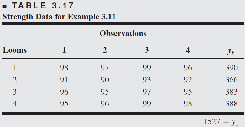
The standard ANOVA partition of the sum of squares is appropriate. There is nothing new in terms of computing.

---

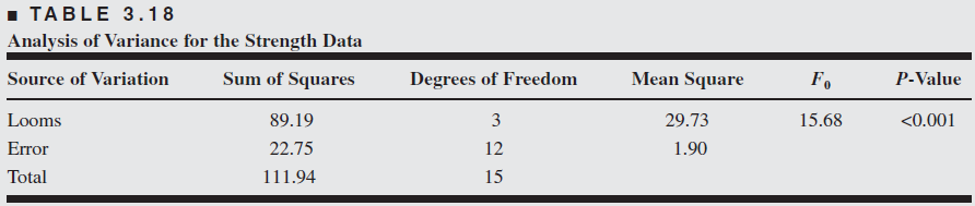
From the ANOVA, we conclude that the looms in the plant differ significantly.

The variance components are estimated by ${\hat{\sigma }}^2=1.90$ and $${\hat{\sigma }}_{\tau }^2=\frac{29.73-1.90}{4}=6.96$$

Therefore, the variance of any observation on strength is estimated by $${\hat{\sigma }}_y={\hat{\sigma }}^2+{\hat{\sigma }}_{\tau }^2=1.90+6.96=8.86.$$ Most of this variability is attributable to differences between looms.

13.2 The Two-Factor Factorial with Random Factors

• Two factors $A$ and $B$, $a$ levels of $A$ and $b$ levels of $B$ are randomly selected in the experiment. The model $$\begin{array}{rl}{y}_{ijk}& =\mu +{\tau }_i+{\beta }_j+(\tau \beta {)}_{ij}+{ϵ}_{ijk},\end{array}$$ where ${\tau }_i$, ${\beta }_j$, $(\tau \beta {)}_{ij}$, and ${ϵ}_{ijk}$ are random

• Assumptions $${\tau }_i\sim \mathcal{N}(0,{\sigma }_{\tau }^2),{\beta }_j\sim \mathcal{N}(0,{\sigma }_{\beta }^2),(\tau \beta {)}_{ij}\sim \mathcal{N}(0,{\sigma }_{\tau \beta }^2),{ϵ}_{ijk}\sim \mathcal{N}(0,{\sigma }^2)$$

• $V\left(y_{ijk}\right)={\sigma }_{\tau }^2+{\sigma }_{\beta }^2+{\sigma }_{\tau \beta }^2+{\sigma }^2$

• Hypotheses of interest $$\begin{array}{rl}(a)& H_0:{\sigma }_{\tau }^2=0\text{against}{H}_1:{\sigma }_{\tau }^2>0\\ (b)& H_0:{\sigma }_{\beta }^2=0\text{against}{H}_1:{\sigma }_{\beta }^2>0\\ (c)& H_0:{\sigma }_{\tau \beta }^2=0\text{against}{H}_1:{\sigma }_{\tau \beta }^2>0\end{array}$$

---

• The form of the test statistics depend on the expected mean squares

• Expected mean squares $$\begin{array}{rl}E(M{S}_A)& ={\sigma }^2+n{\sigma }_{\tau \beta }^2+bn{\sigma }_{\tau }^2\\ E(M{S}_B)& ={\sigma }^2+n{\sigma }_{\tau \beta }^2+an{\sigma }_{\beta }^2\\ E(M{S}_{AB})& ={\sigma }^2+n{\sigma }_{\tau \beta }^2\\ E(M{S}_E)& ={\sigma }^2\end{array}$$

• Test statistic for $H_0:{\sigma }_{\tau \beta }^2=0$ $$F_0=\frac{M{S}_{AB}}{M{S}_E}\sim F_{(a-1)(b-1),ab(n-1)}$$

---

• Expected mean squares $$\begin{array}{rl}E(M{S}_A)& ={\sigma }^2+n{\sigma }_{\tau \beta }^2+bn{\sigma }_{\tau }^2\\ E(M{S}_B)& ={\sigma }^2+n{\sigma }_{\tau \beta }^2+an{\sigma }_{\beta }^2\\ E(M{S}_{AB})& ={\sigma }^2+n{\sigma }_{\tau \beta }^2\\ E(M{S}_E)& ={\sigma }^2\end{array}$$
• Test statistic for $H_0:{\sigma }_{\tau }^2=0$ $$F_0=\frac{M{S}_A}{M{S}_{AB}}\sim F_{(a-1),(a-1)(b-1)}$$

---

• Expected mean squares $$\begin{array}{rl}E(M{S}_A)& ={\sigma }^2+n{\sigma }_{\tau \beta }^2+bn{\sigma }_{\tau }^2\\ E(M{S}_B)& ={\sigma }^2+n{\sigma }_{\tau \beta }^2+an{\sigma }_{\beta }^2\\ E(M{S}_{AB})& ={\sigma }^2+n{\sigma }_{\tau \beta }^2\\ E(M{S}_E)& ={\sigma }^2\end{array}$$
• Test statistic for $H_0:{\sigma }_{\beta }^2=0$ $$F_0=\frac{M{S}_B}{M{S}_{AB}}\sim F_{(b-1),(a-1)(b-1)}$$

---

Notice that these test statistics are not the same as those used if both factors $A$ and $B$ are fixed.

The expected mean squares are always used as a guide to test statistic construction.

In many experiments involving random factors, interest centers at least as much on estimating the variance components as on hypothesis testing.

---

• Estimates of the variance components $$\begin{array}{rl}{\hat{\sigma }}^2& =M{S}_E\\ {\hat{\sigma }}_{\tau \beta }^2& =\frac{M{S}_{AB}-M{S}_E}{n}\\ {\hat{\sigma }}_{\tau }^2& =\frac{M{S}_A-M{S}_E}{bn}\\ {\hat{\sigma }}_{\beta }^2& =\frac{M{S}_B-M{S}_E}{an}\end{array}$$

A Measurement Systems Capability Study

• A Measurement System Capability Study (also called Gauge R&R study, where R&R stands for Repeatability and Reproducibility) is a key part of quality control and process improvement — especially in manufacturing and lab settings.

• Gauge R&R study evaluates how much variation in your measurement data is coming from:

  • The actual process or product you’re measuring

  • The measurement system itself (which includes the instrument and the operator)

• In short, it tells you: “Can we trust our measurement system?”

---

Main Goals

• Assess how precise and reliable your measurements are
• Quantify measurement error
• Determine whether your measurement system is suitable for use in a process control or quality monitoring environment

---

Two Key Components

1. Repeatability Variation when the same operator measures the same item multiple times using the same instrument.

2. Reproducibility Variation between operators (or appraisers), i.e., when different people measure the same item using the same instrument.

---

Basic Experimental Setup

To perform a Gauge R&R study, you typically:

• Choose $n$ parts from the process (covering the process range)

• Have $m$ operators

• Each operator measures each part $r$ times (repeated measures)

---

(Example 13.1)

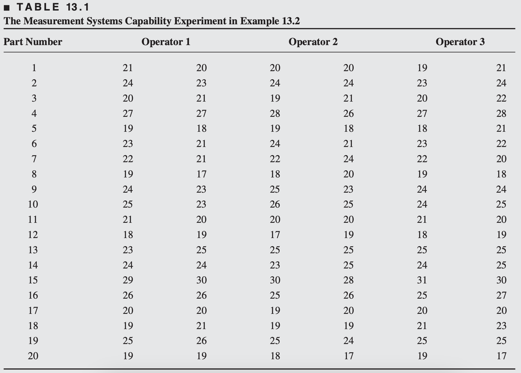
A typical gauge R&R experiment is shown in Table 13.1. An instrument or gauge is used to measure a critical dimension on a part.

Twenty parts have been selected from the production process, and three randomly selected operators measure each part twice with this gauge.

The order in which the measurements are made is completely randomized, so this is a two-factor factorial experiment with design factors parts and operators, with 2 replications.

Both parts and operators are random factors. So, we’re more interested in estimating variance components than testing specific factor levels.

---

---

Let: $$y_{ijk}=\mu +P_i+O_j+(PO{)}_{ij}+{ϵ}_{ijk}$$

Where:

• $y_{ijk}$: the k-th measurement of part $i$ by operator $j$
• $\mu$: overall mean
• $P_i\sim N(0,{\sigma }_P^2)$: random effect of the i-th part
• $O_j\sim N(0,{\sigma }_O^2)$: random effect of the j-th operator
• $(PO{)}_{ij}\sim N(0,{\sigma }_{PO}^2)$: interaction between part and operator
• ${ϵ}_{ijk}\sim N(0,{\sigma }^2)$: repeatability (pure measurement error)

---

---

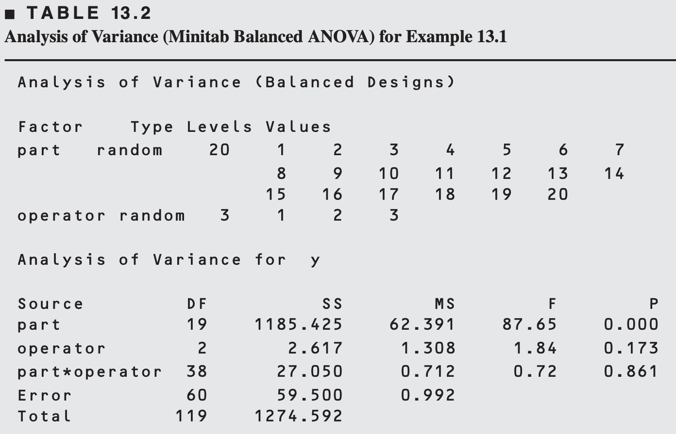
Estimating Variance Components

Using Method of Moments we can estimate:

$$\begin{array}{rl}& {\hat{\sigma }}^2\text{(repeatability)}=0.99\\ & {\hat{\sigma }}_P^2\text{(part variation)}=\frac{62.39-0.71}{(3)(2)}=10.28\\ & {\hat{\sigma }}_O^2\text{(operator variation)}=\frac{1.31-0.71}{(20)(2)}=0.015\\ & {\hat{\sigma }}_{PO}^2\text{(part-operator interaction)}=\frac{0.71-0.99}{2}=-0.14\end{array}$$

---

As interaction is not significant, the reduced model is $y_{ijk}=\mu +P_i+O_j+{ϵ}_{ijk}$

---

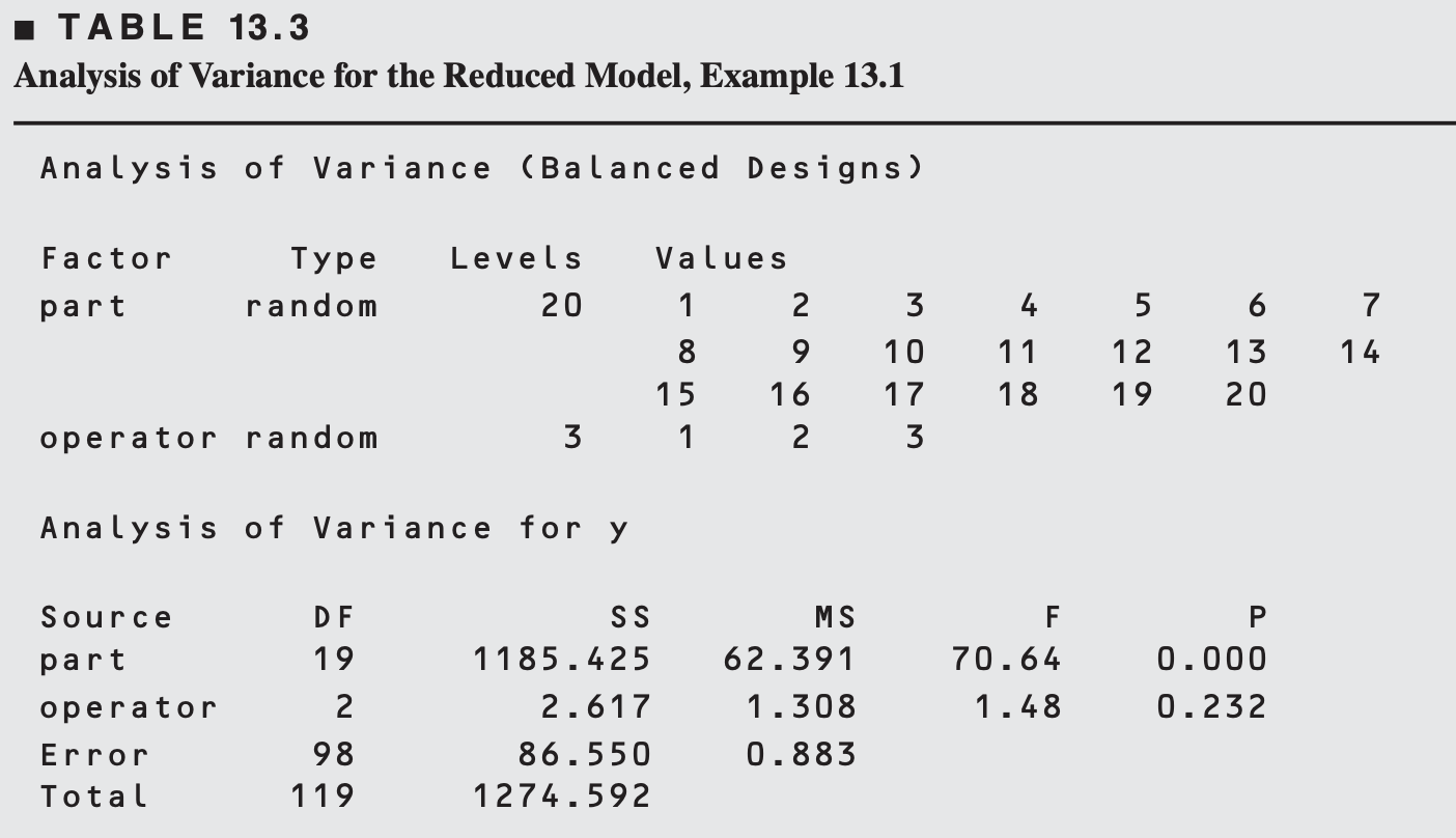
$$\begin{array}{rl}& {\hat{\sigma }}_P^2=\frac{62.39-0.88}{(3)(2)}=10.25\\ & {\hat{\sigma }}_O^2\text{(reproducibility)}=\frac{1.31-0.88}{(20)(2)}=0.0108\\ & {\hat{\sigma }}^2\text{(repeatability)}=0.88\end{array}$$

---

Finally, we could estimate the variance of the gauge as the sum of the variance component estimates ${\hat{\sigma }}^2$ and ${\hat{\sigma }}_O^2$ as $$\begin{array}{rl}{\hat{\sigma }}_{\text{gauge }}^2& ={\hat{\sigma }}^2+{\hat{\sigma }}_O^2\\ & =0.88+0.0108\\ & =0.8908\end{array}$$

The variability in the gauge appears small relative to the variability in the product.

This is generally a desirable situation, implying that the gauge is capable of distinguishing among different grades of product.

13.3 The Two-Factor Mixed Model

• Suppose the levels of the factor $A$ are fixed and the levels of factor $B$ are random
• The two-factor mixed model can be expressed as $$\begin{array}{rl}{y}_{ijk}& =\mu +{\tau }_i+{\beta }_j+(\tau \beta {)}_{ij}+{ϵ}_{ijk},\end{array}$$ where ${\tau }_i$ is fixed, and ${\beta }_j$, $(\tau \beta {)}_{ij}$ and ${ϵ}_{ij}$ are random
• Assumptions $${\beta }_j\sim \mathcal{N}(0,{\sigma }_{\beta }^2),{ϵ}_{ij}\sim \mathcal{N}(0,{\sigma }^2),(\tau \beta {)}_{ij}\sim \mathcal{N}(0,{\sigma }_{\tau \beta }^2(a-1)/a)$$
• Restrictions: $\sum _i{\tau }_i=0$, $\sum _i(\tau \beta {)}_{ij}=0$
• This type of mixed model is known as restricted mixed model

---

• The expected value of the mean squares $$\begin{array}{rl}E(M{S}_A)& ={\sigma }^2+n{\sigma }_{\tau \beta }^2+\frac{bn\sum _i{\tau }_i^2}{a-1}\\ E(M{S}_B)& ={\sigma }^2+an{\sigma }_{\beta }^2\\ E(M{S}_{AB})& ={\sigma }^2+n{\sigma }_{\tau \beta }^2\\ E(M{S}_E)& ={\sigma }^2\end{array}$$
• Test statistic for $H_0:{\tau }_i=0,\mathrm{\forall }i$ $$\begin{array}{rl}{F}_0& =\frac{M{S}_A}{M{S}_{AB}}\sim F_{a-1,(a-1)(b-1)}\end{array}$$

---

• The expected value of the mean squares $$\begin{array}{rl}E(M{S}_A)& ={\sigma }^2+n{\sigma }_{\tau \beta }^2+\frac{bn\sum _i{\tau }_i^2}{a-1}\\ E(M{S}_B)& ={\sigma }^2+an{\sigma }_{\beta }^2\\ E(M{S}_{AB})& ={\sigma }^2+n{\sigma }_{\tau \beta }^2\\ E(M{S}_E)& ={\sigma }^2\end{array}$$
• Test statistic for $H_0:{\sigma }_{\beta }^2=0$ $$\begin{array}{rl}{F}_0& =\frac{M{S}_B}{M{S}_E}\sim F_{b-1,ab(n-1)}\end{array}$$

---

• The expected value of the mean squares $$\begin{array}{rl}E(M{S}_A)& ={\sigma }^2+n{\sigma }_{\tau \beta }^2+\frac{bn\sum _i{\tau }_i^2}{a-1}\\ E(M{S}_B)& ={\sigma }^2+an{\sigma }_{\beta }^2\\ E(M{S}_{AB})& ={\sigma }^2+n{\sigma }_{\tau \beta }^2\\ E(M{S}_E)& ={\sigma }^2\end{array}$$
• Test statistic for $H_0:{\sigma }_{\tau \beta }^2=0$ $$\begin{array}{rl}{F}_0& =\frac{M{S}_{AB}}{M{S}_E}\sim F_{(a-1)(b-1),ab(n-1)}\end{array}$$

---

In the mixed model, it is possible to estimate the fixed factor effects as before which are shown here: $$\begin{array}{rl}& \hat{\mu }={\overline{y}}_{\dots }\\ & {\hat{\tau }}_i={\overline{y}}_{i..}-{\overline{y}}_{\dots }i=1,2,\dots ,a\end{array}$$ The variance components can be estimated using the analysis of variance method by equating the expected mean squares to their observed values: $$\begin{array}{rl}{\hat{\sigma }}_{\beta }^2& =\frac{M{S}_B-M{S}_E}{an}\\ {\hat{\sigma }}_{\tau \beta }^2& =\frac{M{S}_{AB}-M{S}_E}{n}\\ {\hat{\sigma }}^2& =M{S}_E\end{array}$$

---

• Unrestricted mixed models: no restriction of the random effects terms $$\begin{array}{rl}{y}_{ij}& =\mu +{\alpha }_i+{\gamma }_j+(\alpha \gamma {)}_{ij}+{ϵ}_{ijk},\end{array}$$ where ${\alpha }_i$’s are fixed effects such that $\sum _i{\alpha }_i=0$, ${\gamma }_j\sim \mathcal{N}(0,{\sigma }_{\gamma }^2)$, $(\alpha \gamma {)}_{ij}\sim \mathcal{N}(0,{\sigma }_{ij}^2)$, and ${ϵ}_{ij}\sim \mathcal{N}(0,{\sigma }^2)$.
• The expected mean squares $$\begin{array}{rl}E(M{S}_A)& ={\sigma }^2+n{\sigma }_{\alpha \gamma }^2+\frac{bn\sum _i{\alpha }_i^2}{a-1}\\ E(M{S}_B)& ={\sigma }^2+n{\sigma }_{\alpha \gamma }^2+an{\sigma }_{\gamma }^2\\ E(M{S}_{AB})& ={\sigma }^2+n{\sigma }_{\alpha \gamma }^2\\ E(M{S}_E)& ={\sigma }^2\end{array}$$

13.4 Rules for Expected Mean Squares

An important part of experimental design problem is conducting the analysis of variance.

This involves determining the sum of squares for each component in the model and number of degrees of freedom associated with each sum of squares.

To construct appropriate test statistics, the expected mean squares must be determined.

---

By examining the expected mean squares, one may develop the appropriate statistic for testing hypotheses about any model parameter.

The test statistic is a ratio of mean squares that is chosen such that the expected value of the numerator mean square differs from the expected value of the denominator mean square only by the variance component or the fixed factor in which we are interested.

---

• Rule 1. The error term in the model is ${ϵ}_{ij\dots m}$, where the subscript $m$ denotes the replication subscript. For the two-factor model, this rule implies that the error term is ${ϵ}_{ijk}$. The variance component associated with ${ϵ}_{ij\dots m}$ is ${\sigma }^2$.

---

• Rule 2. In addition to an overall mean $(\mu )$ and an error term ${ϵ}_{ij}\dots m$, the model contains all the main effects and any interactions that the experimenter assumes exist. If all possible interactions between $k$ factors exist, then there are $\left(\begin{array}{l}k\\ 2\end{array}\right)$ two-factor interactions, $\left(\begin{array}{l}k\\ 3\end{array}\right)$ three-factor interactions, $\dots ,1k$-factor interaction. If one of the factors in a term appears in parentheses, then there is no interaction between that factor and the other factors in that term.

---

• Rule 3. For each term in the model, divide the subscripts into three classes:

  • live - those subscripts that are present in the term and are not in the parenthesis
    
  • dead - those subscripts that are present in the term and are in the parenthesis
    
  • absent - those subscripts that are present in the model but not in that particular term

E.g. for two-factor fixed effects model, in $(\tau \beta {)}_{ij}$, $i$ and $j$ are live, and $k$ is absent; in ${ϵ}_{(ij)k}$, $k$ is live, and $i$ and $j$ are dead

(We haven’t seen models with dead subscripts, but we will encounter such models later.)

---

• Rule 4. Degrees of freedom. The number of degrees of freedom for any term in the model is the product of the number of levels associated with each dead subscript and the number of levels minus 1 with each live subscript.

E.g. the number of degrees of freedom associated with $(\tau \beta {)}_{ij}$ is $(a-1)(b-1)$, and the number of degrees of freedom associated with ${ϵ}_{(ij)k}$ is $ab(n-1)$.

The number of degrees of freedom for error is obtained by subtracting the sum of all other degrees of freedom from $N-1$, where $N$ is the total number of observations.

---

• Rule 5. Each term in the model has either a variance component (random effect) or a fixed factor (fixed effect) associated with it.

If the interaction term contain at least one random effect, the entire effect is termed is considered as random

A variance component has Greek letters as subscripts to identify the particular random effect, e.g. ${\sigma }_{\beta }^2$ is the variance component corresponding to random factor $B$

A fixed effect always represented by the sum of squares of the model components associated with that factor divided by its degrees of freedom, e.g. $\sum _i{\tau }_i^2/(a-1)$ for factor $A$ when it is fixed

---

• Rule 6. There is an expected mean square for each model component. The expected mean square for error is $E\left({MS}_E\right)={\sigma }^2$.

In case of the restricted model, for every other model term, the expected mean square contains

• ${\sigma }^2$ plus
• either the variance component or the fixed effect component for that term, plus
• those components for all other model terms that contain the effect in question and that involve no interactions with other fixed effects.

The coefficient of each variance component or fixed effect is the number of observations at each distinct value of that component.

---

To illustrate for the case of the two-factor fixed effects model, consider finding the interaction expected mean square, $E\left(M{S}_{AB}\right)$.

• The expected mean square will contain only the fixed effect for the $AB$ interaction (because no other model terms contain $AB$) plus ${\sigma }^2$, and the fixed effect for $AB$ will be multiplied by $n$ because there are $n$ observations at each distinct value of the interaction component (the $n$ observations in each cell).
• Thus, the expected mean square for $AB$ is $$E\left(M{S}_{AB}\right)={\sigma }^2+\frac{n\sum _{i=1}^a\sum _{j=1}^b(\tau \beta {)}_{ij}^2}{(a-1)(b-1)}$$

---

• As another illustration of the two-factor fixed effects model, the expected mean square for the main effect of $A$ would be $$E\left(M{S}_A\right)={\sigma }^2+\frac{bn\sum _{i=1}^a{\tau }_i^2}{(a-1)}$$ The multiplier in the numerator is $bn$ because there are $bn$ observations at each level of $A$. The $AB$ interaction term is not included in the expected mean square because while it does include the effect in question $(A)$, factor $B$ is a fixed effect.

---

To illustrate how Rule 6 applies to a model with random effects, consider the two-factor random model. The expected mean square for the $AB$ interaction would be $$E\left(M{S}_{AB}\right)={\sigma }^2+n{\sigma }_{\tau \beta }^2$$ and the expected mean square for the main effect of $A$ would be $$E\left(M{S}_A\right)={\sigma }^2+n{\sigma }_{\tau \beta }^2+bn{\sigma }_{\tau }^2$$ Note that the variance component for the $AB$ interaction term is included because $A$ is included in $AB$ and $B$ is a random effect.

---

Two factor fixed effects model $$\begin{array}{c}E\left(M{S}_A\right)={\sigma }^2+\frac{bn\sum _{i=1}^a{\tau }_i^2}{(a-1)}\\ E\left(M{S}_B\right)={\sigma }^2+\frac{an\sum _{j=1}^b{\beta }_j^2}{b-1}\\ E\left(M{S}_{AB}\right)={\sigma }^2+\frac{n\sum _{i=1}^a\sum _{j=1}^b(\tau \beta {)}_{ij}^2}{(a-1)(b-1)}\\ E\left(M{S}_E\right)={\sigma }^2\end{array}$$

---

Two factor random model $$\begin{array}{rl}E\left(M{S}_A\right)& ={\sigma }^2+n{\sigma }_{\tau \beta }^2+bn{\sigma }_{\tau }^2\\ E\left(M{S}_B\right)& ={\sigma }^2+n{\sigma }_{\tau \beta }^2+an{\sigma }_{\beta }^2\\ E\left(M{S}_{AB}\right)& ={\sigma }^2+n{\sigma }_{\tau \beta }^2\\ E\left(M{S}_E\right)& ={\sigma }^2\end{array}$$

---

Restricted form of two factor mixed model $$\begin{array}{rl}E\left(M{S}_A\right)& ={\sigma }^2+n{\sigma }_{\tau \beta }^2+\frac{bn\sum _{i=1}^a{\tau }_i^2}{a-1}\\ E\left(M{S}_B\right)& ={\sigma }^2+an{\sigma }_{\beta }^2\\ E\left(M{S}_{AB}\right)& ={\sigma }^2+n{\sigma }_{\tau \beta }^2\\ E\left(M{S}_E\right)& ={\sigma }^2\end{array}$$

---

Rule 6 can be easily modified to give expected mean squares for the unrestricted form of the mixed model. Simply include the term for the effect in question, plus all the terms that contain this effect as long as there is at least one random factor.

Unrestricted form of two factor mixed model.

$$\begin{array}{rl}E\left(M{S}_A\right)& ={\sigma }^2+n{\sigma }_{\tau \beta }^2+\frac{bn\sum _{i=1}^a{\tau }_i^2}{a-1}\\ E\left(M{S}_B\right)& ={\sigma }^2+n{\sigma }_{\tau \beta }^2+an{\sigma }_{\beta }^2\\ E\left(M{S}_{AB}\right)& ={\sigma }^2+n{\sigma }_{\tau \beta }^2\\ E\left(M{S}_E\right)& ={\sigma }^2\end{array}$$

13.5 Approximate F-Tests

Consider a three-factor factorial experiment with a levels of factor $A$, $b$ levels of factor $B$, $c$ levels of factor $C$, and $n$ replicates.

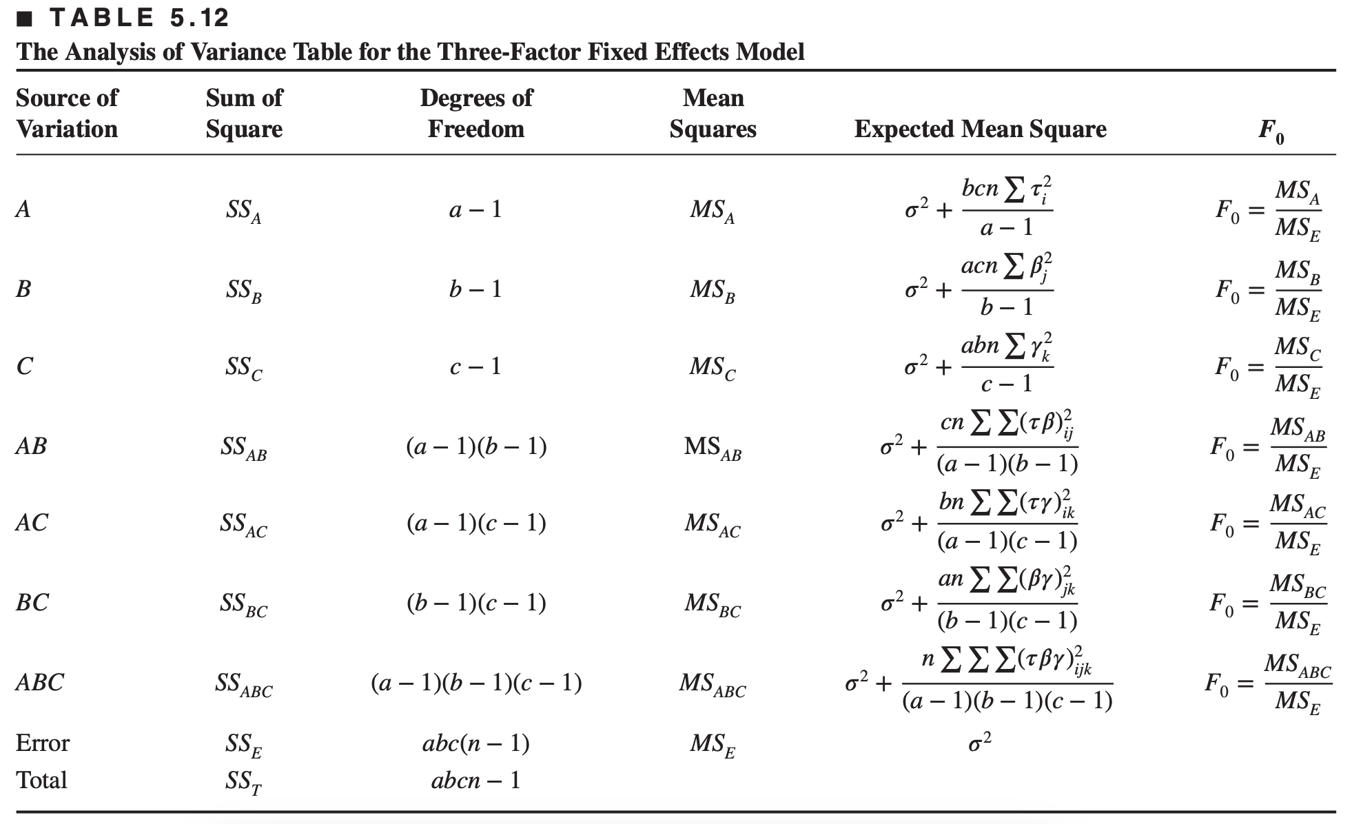
First, assume that all the factors are fixed. $$\begin{array}{rl}{y}_{ijkl}=& \mu +{\tau }_i+{\beta }_j+{\gamma }_k+(\tau \beta {)}_{ij}+(\tau \gamma {)}_{ik}+(\beta \gamma {)}_{jk}\\ & +(\tau \beta \gamma {)}_{ijk}+{ϵ}_{ijkl}\{\begin{array}{c}i=1,2,\dots ,a\\ j=1,2,\dots ,b\\ k=1,2,\dots ,c\\ l=1,2,\dots ,n\end{array}\end{array}$$ Then the analysis of this design is given below

---

---

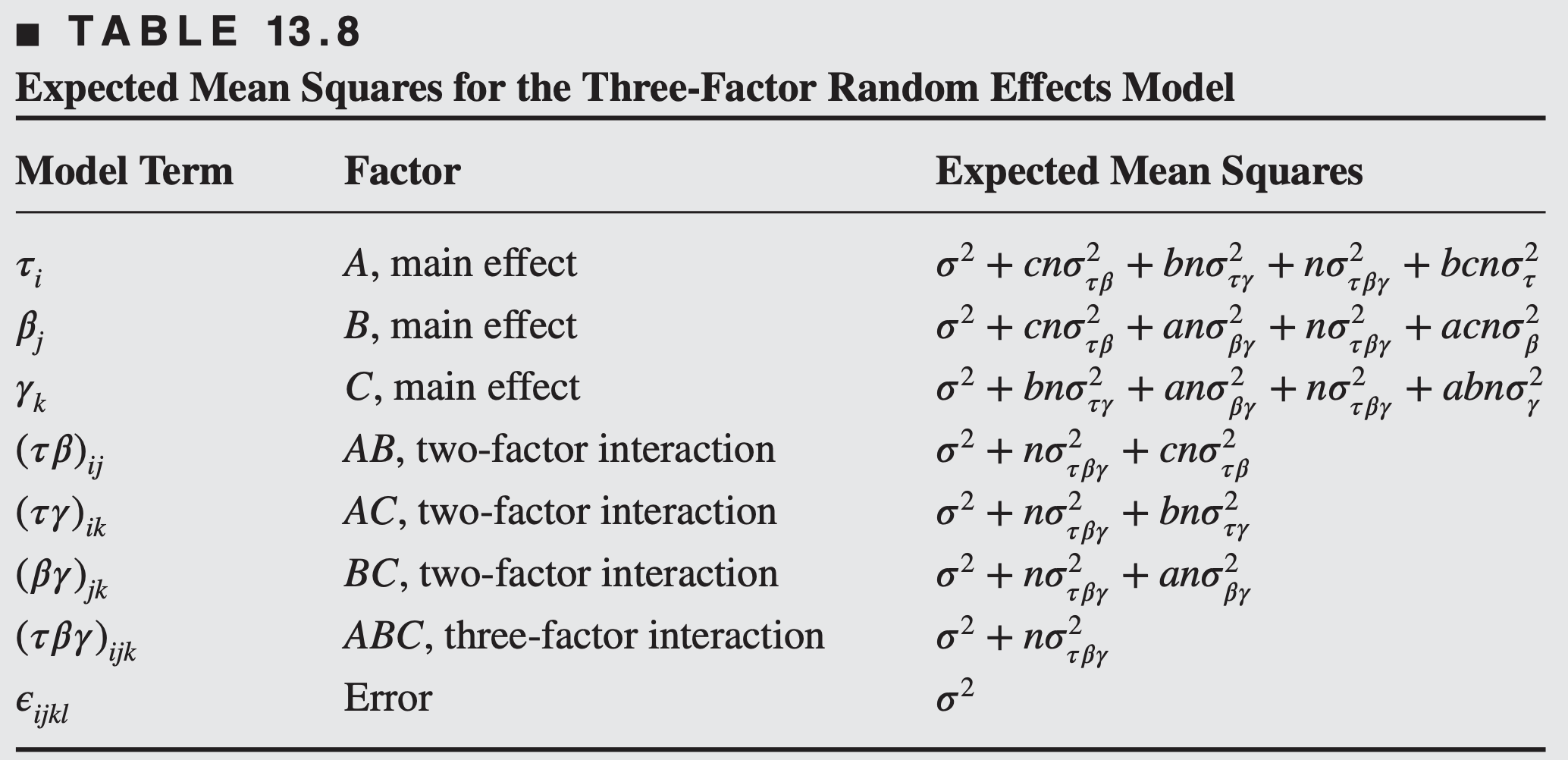
Now, assume that all the three factors are random. The three-factor random effects model is $$\begin{array}{rl}{y}_{ijkl}& ={\tau }_i+{\beta }_j+{\gamma }_k+(\tau \beta {)}_{ij}+(\tau \gamma {)}_{ik}+(\beta \gamma {)}_{jk}\\ & +(\tau \beta \gamma {)}_{ijk}+{ϵ}_{ijkl}\end{array}$$ Assumptions:

• ${\tau }_i\sim \mathcal{N}(0,{\sigma }_{\tau }^2)$, ${\beta }_j\sim \mathcal{N}(0,{\sigma }_{\beta }^2)$, ${\gamma }_k\sim \mathcal{N}(0,{\sigma }_{\gamma }^2)$
• $(\tau \beta {)}_{ij}\sim \mathcal{N}(0,{\sigma }_{\tau \beta }^2)$, $(\tau \gamma {)}_{ik}\sim \mathcal{N}(0,{\sigma }_{\tau \gamma }^2)$, $(\beta \gamma {)}_{jk}\sim \mathcal{N}(0,{\sigma }_{\beta \gamma }^2)$
• $(\tau \beta \gamma {)}_{ijk}\sim \mathcal{N}(0,{\sigma }_{\tau \beta \gamma }^2)$
• ${ϵ}_{ijk}\sim \mathcal{N}(0,{\sigma }^2)$
• All the random effects are pair-wise independent

---

The expected mean squares assuming that all the factors are random are

• What is the test statistic for $H_0:{\sigma }_{\tau }^2=0$?

---

• For three-factor random effects model, no exact test statistic for testing certain effects, e.g.  for $H_0:{\sigma }_{\tau }^2=0$ one possible test statistic $$\begin{array}{rl}{F}_0& =\frac{{\text{MS}}_A}{{\text{MS}}_{ABC}}\\ & =\frac{{\sigma }^2+cn{\sigma }_{\tau \beta }^2+bn{\sigma }_{\tau \gamma }^2+n{\sigma }_{\tau \beta \gamma }^2+bcn{\sigma }_{\tau }^2}{{\sigma }^2+n{\sigma }_{\tau \beta \gamma }^2},\end{array}$$ which would be useful if the interactions ${\sigma }_{\tau \beta }^2$ and ${\sigma }_{\tau \gamma }^2$ are negligible.

---

• If we cannot assume that the certain interactions are negligible and we need to make inferences about those effects for which exact tests do not exist, Satterthwaite’ method can be used.

• Satterthwaite’s method uses the linear combinations of mean squares, for example $$\begin{array}{rl}& M{S}^{\prime }=M{S}_r+\cdots +M{S}_s\\ & M{S}^{\prime \prime }=M{S}_u+\cdots +M{S}_v\end{array}$$ are chosen so that $E\left({MS}^{\prime }\right)-E(MS\prime \prime )$ is equal to a multiple of the effect (the model parameter or variance component) considered in the null hypothesis.

---

Then the test statistic would be $$F=\frac{M{S}^{\prime }}{M{S}^{\prime \prime }}$$ which is distributed approximately as $F_{p,q}$, where $$p=\frac{{(M{S}_r+\cdots +M{S}_s)}^2}{M{S}_r^2/f_r+\cdots +M{S}_s^2/f_s}$$ $$q=\frac{{(M{S}_u+\cdots +M{S}_v)}^2}{M{S}_u^2/f_u+\cdots +M{S}_v^2/f_v}$$ In $p$ and $q$, $f_i$ is the number of degrees of freedom associated with the mean square ${MS}_i$

E.g.

E.g. For our example, for testing the null hypothesis, $H_0:{\sigma }_{\tau }^2=0$, we can use the test statistic $$\begin{array}{rl}F& =\frac{M{S}_A+M{S}_{ABC}}{M{S}_{AB}+M{S}_{AC}}\\ & =\frac{2{\sigma }^2+cn{\sigma }_{\tau \beta }^2+bn{\sigma }_{\tau \gamma }^2+2n{\sigma }_{\tau \beta \gamma }^2+bcn{\sigma }_{\tau }^2}{2{\sigma }^2+2{\sigma }_{\tau \beta \gamma }^2+bn{\sigma }_{\tau \gamma }^2+cn{\sigma }_{\tau \beta }^2}\end{array}$$

---

• Under $H_0$, the statistic $F$ follows $F$-distribution with $p$ and $q$ degrees of freedom, where $$\begin{array}{r}p=\frac{(M{S}_A+M{S}_{ABC}{)}^2}{(M{S}_A^2/f_A)+(M{S}_{ABC}^2/f_{ABC})}\\ q=\frac{(M{S}_{AB}+M{S}_{AC}{)}^2}{(M{S}_{AB}^2/f_{AB})+(M{S}_{AC}^2/f_{AC})}\end{array}$$ and $f_A$ is degrees of freedom associated with $M{S}_A$.