Chapter 14

(AST301) Design and Analysis of Experiments II

14 Nested and Split-Plot Designs

This chapter introduces two important types of experimental designs, the nested design and the split-plot design.

Both of these designs find reasonably widespread application in the industrial use of designed experiments.

They also frequently involve one or more random factors, and so some of the concepts introduced in Chapter 13 will find application here.

14.1 The Two-Stage Nested Design

• In a nested design, the levels of one factor $(B)$ is similar to but not identical to each other at different levels of another factor ($A$)

• Consider a company that purchases material from three suppliers

  • The material comes in batches
  • Is the purity of the material uniform?

• Experimental design

  • Select four batches at random from each supplier
  • Make three purity determinations from each batch

---

---

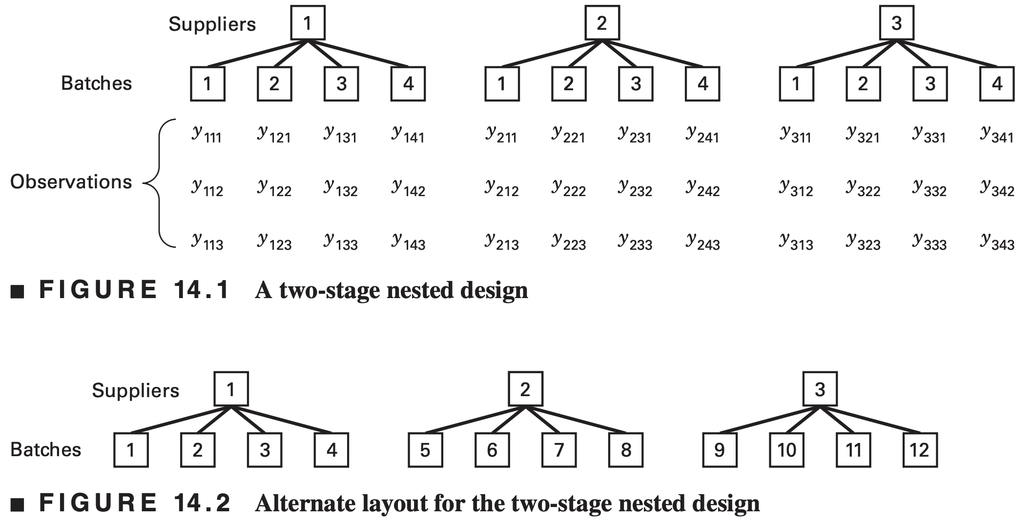
• If this were a factorial, then batch 1 would always refer to the same batch, batch 2 would always refer to the same batch, and so on. This is clearly not the case because the batches from each supplier are unique for that particular supplier.

• Sometimes we may not know whether a factor is crossed in a factorial arrangement or nested. If the levels of the factor can be renumbered arbitrarily as in Figure 14.2, then the factor is nested.

Statistical Analysis

• Statistical model for two-stage nested design $$\begin{array}{rl}{y}_{ijk}& =\mu +{\tau }_i+{\beta }_{j(i)}+{ϵ}_{(ij)k}\{\begin{array}{c}i=1,\dots ,a\\ j=1,\dots ,b\\ k=1,\dots ,n\end{array}\end{array}$$

The notation $j(i)$ indicates that the $jth$ level of factor $B$ is nested under the $ith$ level of factor $A$

• Factors $A$ and $B$ could be fixed and/or random
• This is a balanced nested design as equal number of levels of $B$ within each level of $A$ and equal number of replicates.
• No interaction

---

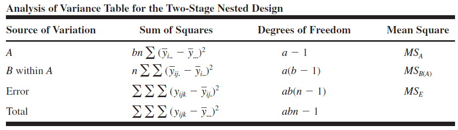
• Decomposition of sum of squares $$\begin{array}{rl}\sum _i\sum _j\sum _k(y_{ijk}-{\overline{y}}_{\cdot \cdot \cdot }{)}^2& =\sum _i\sum _j\sum _k\{({\overline{y}}_{i\cdot \cdot }-{\overline{y}}_{\cdot \cdot \cdot })+({\overline{y}}_{ij\cdot }-{\overline{y}}_{i\cdot \cdot })\\ & +(y_{ijk}-{\overline{y}}_{ij\cdot }){\}}^2\\ & =bn\sum _i({\overline{y}}_{i\cdot \cdot }-{\overline{y}}_{\cdot \cdot \cdot }{)}^2+n\sum _{i,j}({\overline{y}}_{ij\cdot }-{\overline{y}}_{i\cdot \cdot }{)}^2\\ & \sum _{i,j,k}(y_{ijk}-{\overline{y}}_{ij\cdot }{)}^2\\ S{S}_T& =S{S}_A+S{S}_{B(A)}+S{S}_E\end{array}$$

• What are the corresponding degrees of freedom and expressions of mean squares?

---

$$\begin{array}{c}S{S}_T=S{S}_A+S{S}_{B(A)}+S{S}_E\\ df:abn-1=a-1+a(b-1)+ab(n-1)\end{array}$$

If the errors are $\mathrm{NID}(0,{\sigma }^2)$, we may divide each sum of squares on the right of the above equation by its degrees of freedom to obtain independently distributed mean squares such that the ratio of any two mean squares is distributed as $F$.

---

The appropriate statistics for testing the effects of factors $A$ and $B$ depend on whether $A$ and $B$ are fixed or random.

If factors $A$ and $B$ are fixed, we assume that ${\mathrm{\Sigma }}_{i=1}^a{\tau }_i=0$ and ${\mathrm{\Sigma }}_{j=1}^b{\beta }_{j(i)}=0(i=1,2,\dots ,a)$.

That is, the $A$ treatment effects sum to zero, and the $B$ treatment effects sum to zero within each level of $A$.

---

If $A$ and $B$ are random, we assume that ${\tau }_i$ is $\mathrm{NID}(0$, ${\sigma }_{\tau }^2)$ and ${\beta }_{j(i)}$ is $NID(0,{\sigma }_{\beta }^2)$.

Mixed models with $A$ fixed and $B$ random are also widely encountered. The expected mean squares can be determined by a straightforward application of the rules in Chapter 13.

The expected mean squares for these three situations is given in the next table.

---

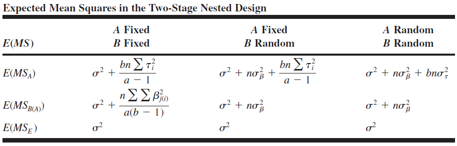
• If the levels of $A$ and $B$ are fixed,
  • $H_0:{\tau }_i=0$ is tested by ${MS}_A/{MS}_E$ and
  • $H_0:{\beta }_{j(i)}=0$ is tested by ${MS}_{B(A)}/{MS}_E$
• If $A$ is a fixed factor and $B$ is random,
  • $H_0:{\tau }_i=0$ is tested by ${MS}_A/{MS}_{B(A)}$ and
  • $H_0:{\sigma }_{\beta }^2=0$ is tested by ${MS}_{B(A)}/{MS}_E$
• Finally, if both $A$ and $B$ are random factors,
  • $H_0:{\sigma }_{\tau }^2=0$ is tested by ${MS}_A/{MS}_{B(A)}$ and
  • $H_0:{\sigma }_{\beta }^2=0$ is tested by ${MS}_{B(A)}/{MS}_E$

---

Computing formulas for the sums of squares are given below

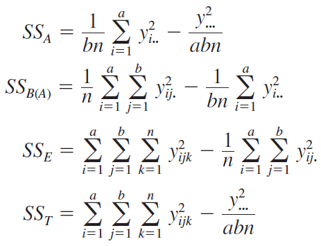
Example 14.1

Consider a company that buys raw material in batches from three different suppliers. The purity of this raw material varies considerably, which causes problems in manufacturing the finished product. We wish to determine whether the variability in purity is attributable to differences between the suppliers. Four batches of raw material are selected at random from each supplier, and three determinations of purity are made on each batch.

This is, of course, a two-stage nested design. The data, after coding by subtracting 93, are shown below.

---

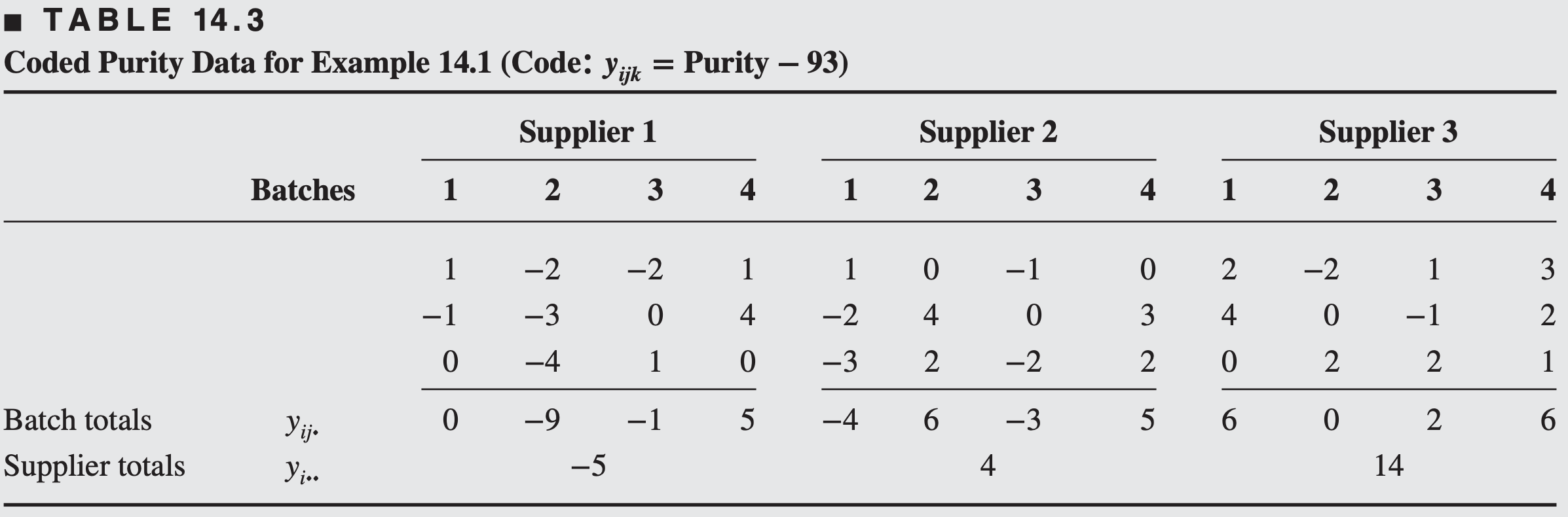
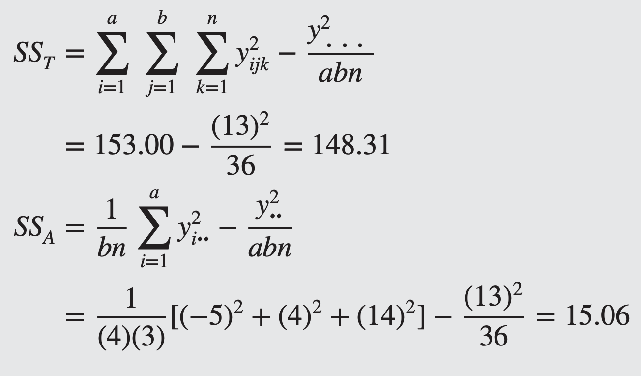
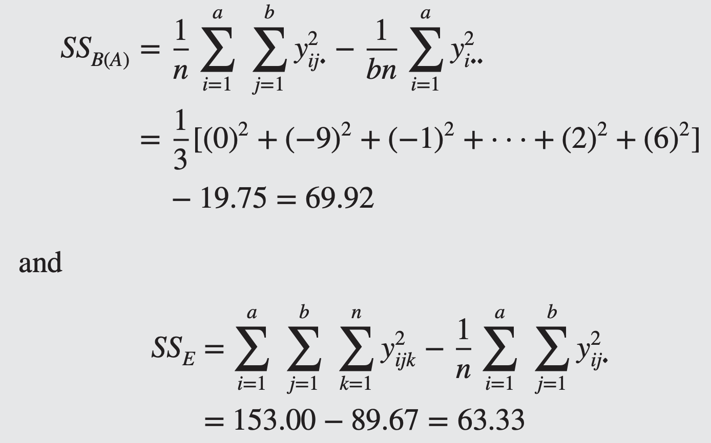
The sums of squares are computed as follows

---

---

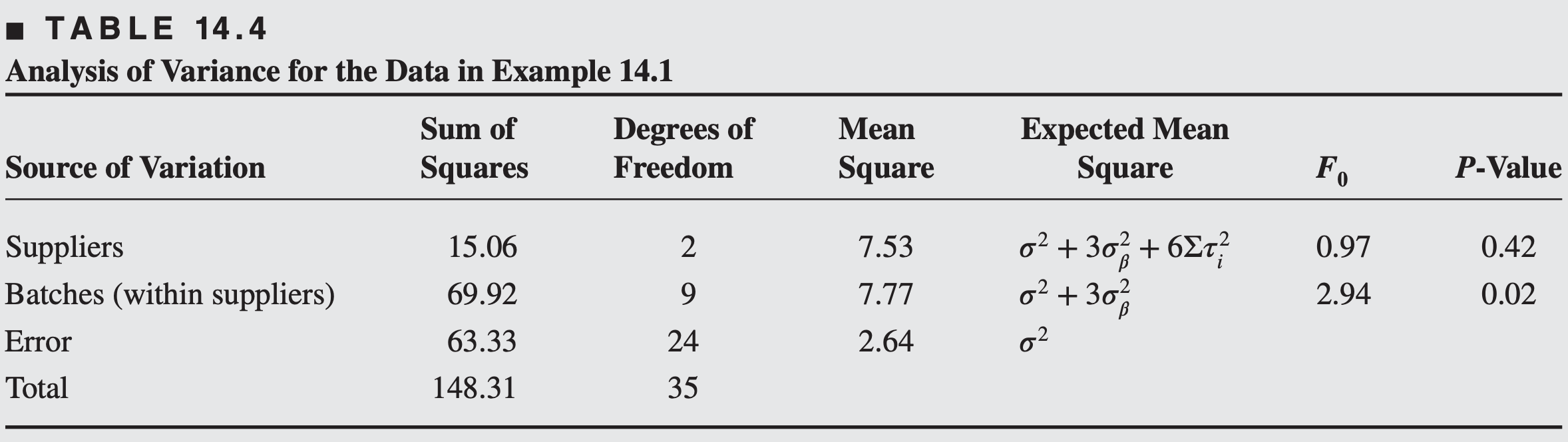
• There is no difference in purity among suppliers, but significant difference in purity among batches (within suppliers)

Diagnostic checking

• For the model $y_{ijk}=\mu +{\tau }_i+{\beta }_{j(i)}+{ϵ}_{ijk}$, the estimates of parameters are $$\hat{\mu }={\overline{y}}_{\cdot \cdot \cdot },{\hat{\tau }}_i={\overline{y}}_{i\cdot \cdot }-{\overline{y}}_{\cdot \cdot \cdot },{\hat{\beta }}_{j(i)}={\overline{y}}_{ij\cdot }-{\overline{y}}_{i\cdot \cdot }$$

• The fitted model ${\hat{y}}_{ijk}=\hat{\mu }+{\hat{\tau }}_i+{\hat{\beta }}_{j(i)}={\overline{y}}_{ij\cdot }$

• The residuals ${\widehat{ϵ}}_{ijk}=y_{ijk}-{\hat{y}}_{ijk}$

• ANOVA indicates that there is statistically significant batch-to-batch variability. But, is the variability within batches the same for all suppliers? The plot of residuals versus supplier can help us answer this.

Estimates of Variance Components

For the random effects case, the analysis of variance method can be used to estimate the variance components ${\sigma }^2,{\sigma }_{\tau }^2$, and ${\sigma }_{\beta }^2$. Applying the ANOVA method, we obtain $$\begin{array}{rl}{\hat{\sigma }}^2& =M{S}_E\\ {\hat{\sigma }}_{\beta }^2& =\frac{M{S}_{B(A)}-M{S}_E}{n}\\ {\hat{\sigma }}_{\tau }^2& =\frac{M{S}_A-M{S}_{B(A)}}{bn}\end{array}$$

---

Many applications of nested designs involve a mixed model, with the main factor $(A)$ fixed and the nested factor $(B)$ random. This is the case for the problem described in Example 14.1, where suppliers (factor $A$) are fixed, and batches of raw material (factor $B$) are random. The effects of the suppliers may be estimated by $$\begin{array}{rl}& {\hat{\tau }}_1={\overline{y}}_{1..}-{\overline{y}}_{\dots }=\frac{-5}{12}-\frac{13}{36}=\frac{-28}{36}\\ & {\hat{\tau }}_2={\overline{y}}_{2..}-{\overline{y}}_{\dots }=\frac{4}{12}-\frac{13}{36}=\frac{-1}{36}\\ & {\hat{\tau }}_3={\overline{y}}_{3..}-{\overline{y}}_{\dots }=\frac{14}{12}-\frac{13}{36}=\frac{29}{36}\end{array}$$

---

We estimate the variance components as $$\begin{array}{c}{\hat{\sigma }}^2=M{S}_E=2.64\\ {\hat{\sigma }}_{\beta }^2=\frac{M{S}_{B(A)}-M{S}_E}{n}=\frac{7.77-2.64}{3}=1.71\end{array}$$

From the analysis in Example 14.1 (in Table 14.4), we know that the ${\tau }_i$ does not differ significantly from zero, whereas the variance component ${\sigma }_{\beta }^2$ is greater than zero.

14.2 The General $m$-Stage Nested Design

Suppose a foundry wishes to investigate the hardness of two different formulations of a metal alloy. Three heats of each alloy formulation are prepared, two ingots are selected at random from each heat for testing, and two hardness measurements are made on each ingot. In this experiment, heats are nested under the levels of the factor alloy formulation, and ingots are nested under the levels of the factor heats. Thus, this is a three-stage nested design with two replicates.

---

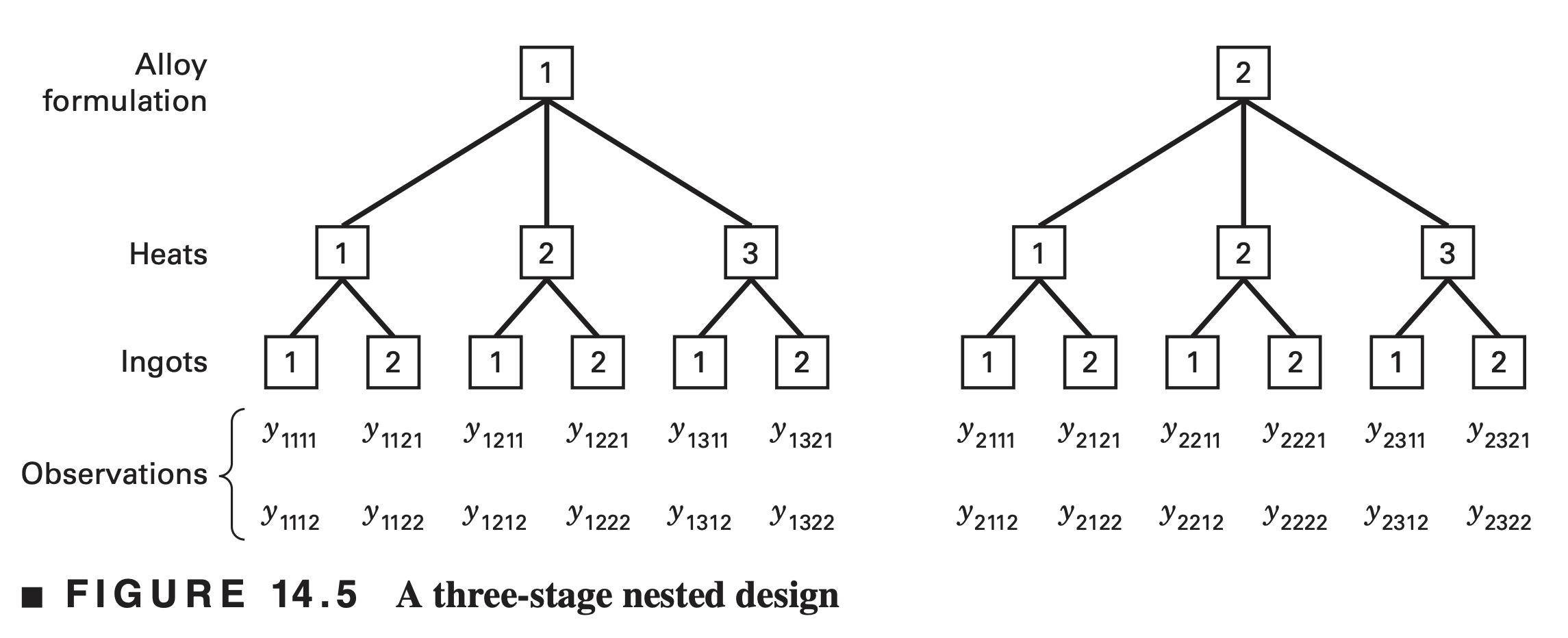
The model for the general three stage nested design is $$y_{ijkl}=\mu +{\tau }_i+{\beta }_{j(i)}+{\gamma }_{k(ij)}+{ϵ}_{(ijk)l}\{\begin{array}{l}i=1,2,\dots ,a\\ j=1,2,\dots ,b\\ k=1,2,\dots ,c\\ l=1,2,\dots ,n\end{array}$$ For our example,

• ${\tau }_i$ is the effect of the $i$th alloy formulation,
• ${\beta }_{j(i)}$ is the effect of the $j$th heat within the $i$th alloy,
• ${\gamma }_{k(ij)}$ is the effect of the $k$th ingot within the $j$th heat and $i$th alloy, and
• ${ϵ}_{(ijk)l}$ is the usual $\mathrm{NID}(0,{\sigma }^2)$ error term.

Exercise

Given a three-stage nested design $$y_{ijkl}=\mu +{\tau }_i+{\beta }_{j(i)}+{\gamma }_{k(ij)}+{ϵ}_{ijkl}$$

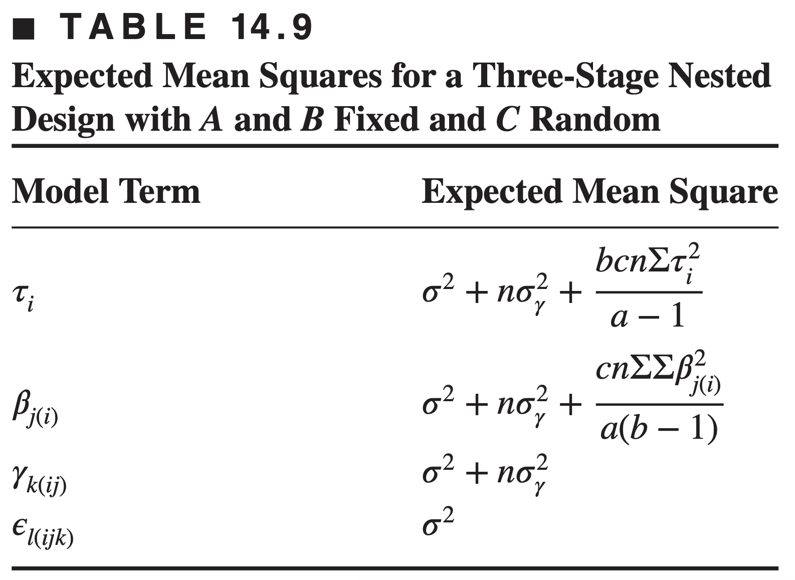
• Find degrees of freedom and expressions of expected mean squares for the following situations:

  • All the factors $A$, $B$, and $C$ are fixed
  • Factors $A$ and $B$ are fixed, and $C$ is random
  • Factor $A$ is fixed, and $B$ and $C$ are random

---

14.3 Designs with Both Nested and Factorial Factors

Occasionally in a multifactor experiment, some factors are arranged in a factorial layout and other factors are nested.

We sometimes call these designs nested–factorial designs. The statistical analysis of one such design with three factors is illustrated in the following example.

---

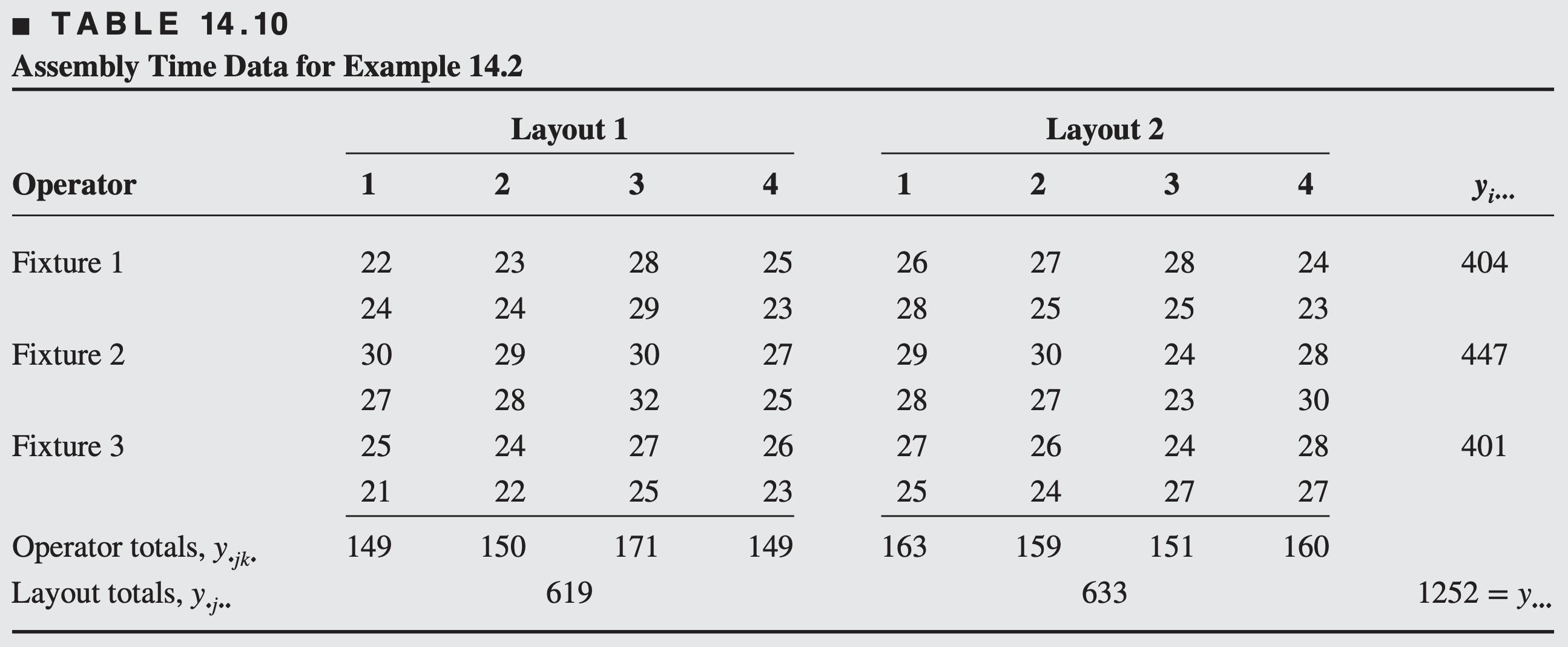
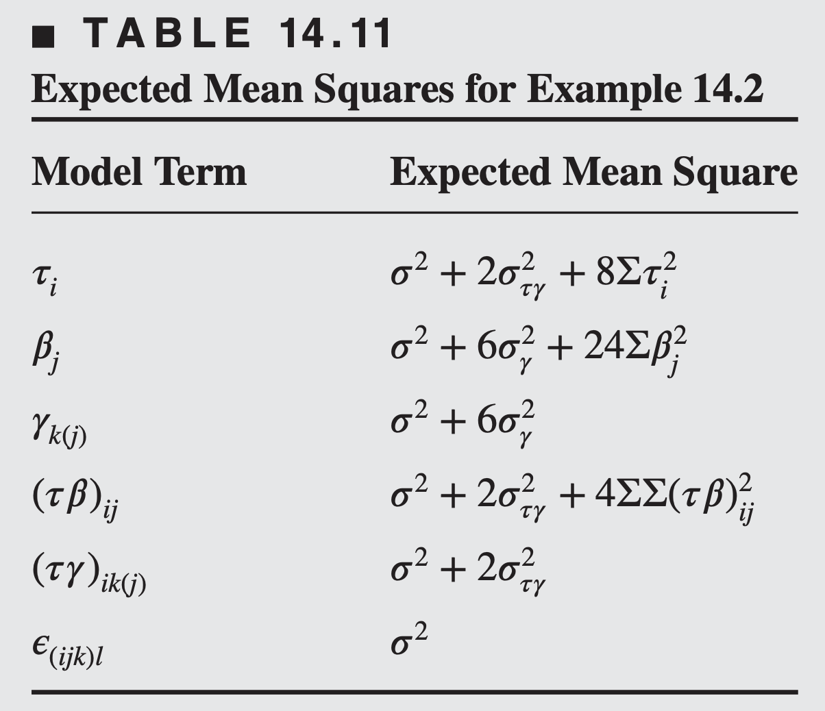
$$y_{ijkl}=\mu +{\tau }_i+{\beta }_j+{\gamma }_{k(j)}+(\tau \beta {)}_{ij}+(\tau \gamma {)}_{ik(j)}+{ϵ}_{(ijk)l}\{\begin{array}{l}i=1,2,3\\ j=1,2\\ k=1,2,3,4\\ l=1,2\end{array}$$

---

Assume that fixtures and layouts are fixed, operators are random – gives a mixed model (use restricted form)

14.4 Split-plot design

• The split-plot is a multifactor experiment where it is not possible to completely randomize the order of the runs

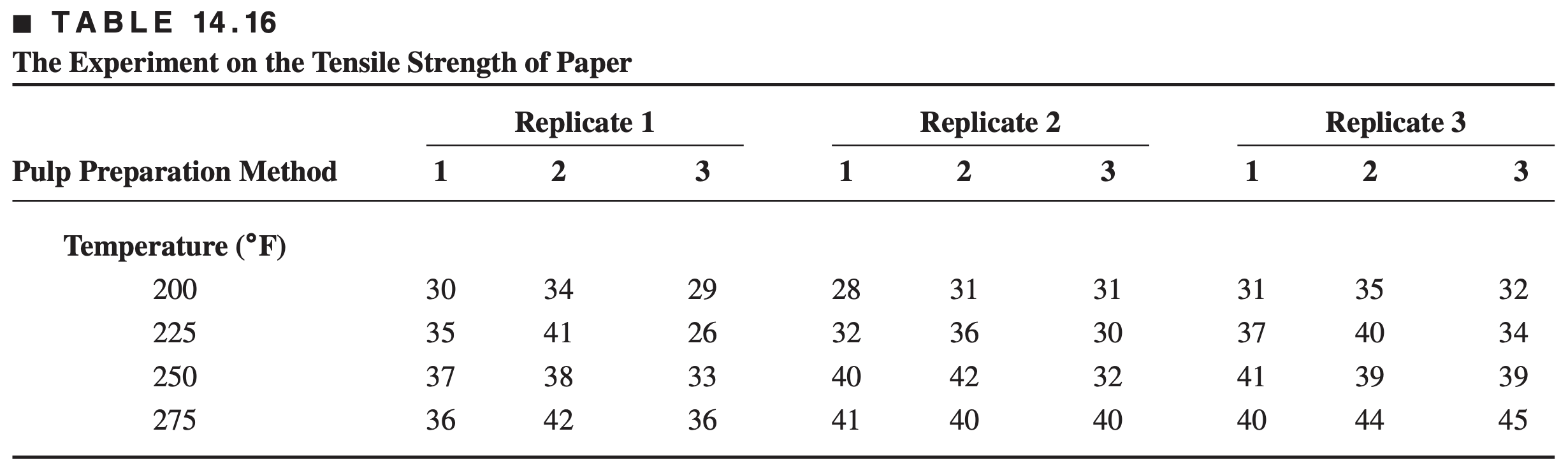
• A paper manufacturer is interested in examining the effect of pulp preparation method and cooking temperature on the tensile strength of the paper

  • Three pulp preparation methods
  • Four different temperatures
  • Each replicate requires 12 runs
  • The experimenters want to use three replicates
  • How many batches of pulp are required?

---

• Pulp preparation methods is a hard-to-change factor

Consider an alternate experimental design:

1. In replicate 1: select a pulp preparation method, prepare a batch

• Divide the batch into four sections or samples, and assign one of the temperature levels to each
• Repeat for each pulp preparation method

2. Conduct replicates 2 similarly
3. Conduct replicates 3 similarly

---

• Each replicate (sometimes called blocks) has been divided into three parts, called the whole plots

• Pulp preparation methods is the whole plot treatment

• Each whole plot has been divided into four subplots or split-plots

• Temperature is the subplot treatment

• Generally, the hard-to-change factor is assigned to the whole plots

• This design requires only 9 batches of pulp (assuming three replicates)

---

---

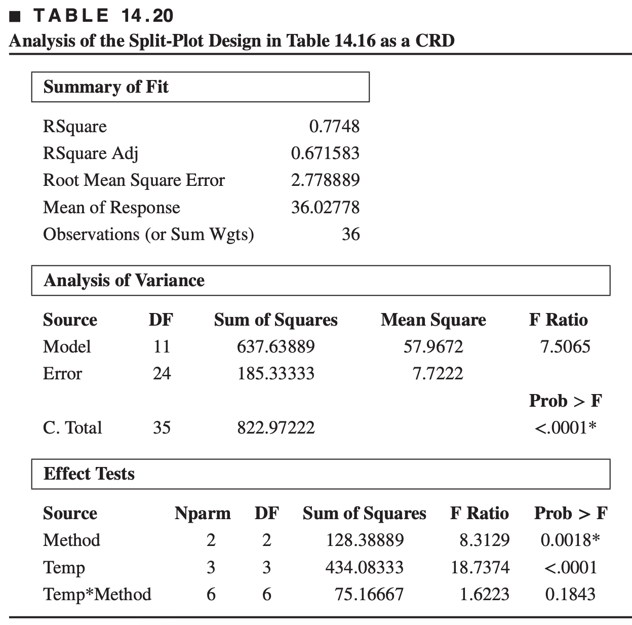
• This is not a randomized block design with three levels of pulp preparation and four levels of cooking temperature (why?)

• To be a randomized block design the order of the experiments within a block should be completely randomized which is not the case for our example where we only randomize the order of cooking temperature within a pulp preparation

• This design is known as split-plot design where each replicate (block) is divided into three whole plots (pulp preparation) and each whole plot is divided into four subplots (cooking temperature)

• Since the whole plot treatments are confounded with whole plot where as subplots are not confounded, so treatment of interest best to assign into subplots, if possible

---

• Split-plot design can be viewed as two experiments combined or superimposed on each other

• One experiment has the whole plot factor applied to the large experimental units (factor whose level is hard to change) and the other experiment has the subplot factor applied to the smaller units (factor whose level is easy to change)

• In general split-plot within a whole plot will be more similar than split plots in different whole plots.

• Within whole plot, comparisons will generally be more precise than between whole plot comparisons, i.e. estimates of $B$ and $AB$ will be more precise compared to the estimates of $A$

• If the levels of all factors are easy to change, split-plot designs are recommended only when there is a considerable less interest in one or more of the treatment factors

Analysis of Split-plot design

• In the statistical analysis of split-plot designs, we must take into account the presence of two different sizes of experimental units used to test the effect of whole plot treatment and split-plot treatment.

• Factor $A$ effects are estimated using the whole plots and factor $B$ and the $A\ast B$ interaction effects are estimated using the split plots.

---

The linear model for the split-plot design is $$\begin{array}{rl}{y}_{ijk}=& \mu +{\tau }_i+{\beta }_j+(\tau \beta {)}_{ij}+{\gamma }_k+(\tau \gamma {)}_{ik}\\ & +(\beta \gamma {)}_{jk}+(\tau \beta \gamma {)}_{ijk}+{ϵ}_{ijk}\{\begin{array}{rl}& i=1,2,\dots ,r\\ & j=1,2,\dots ,a\\ & k=1,2,\dots ,b\end{array}\end{array}$$ where

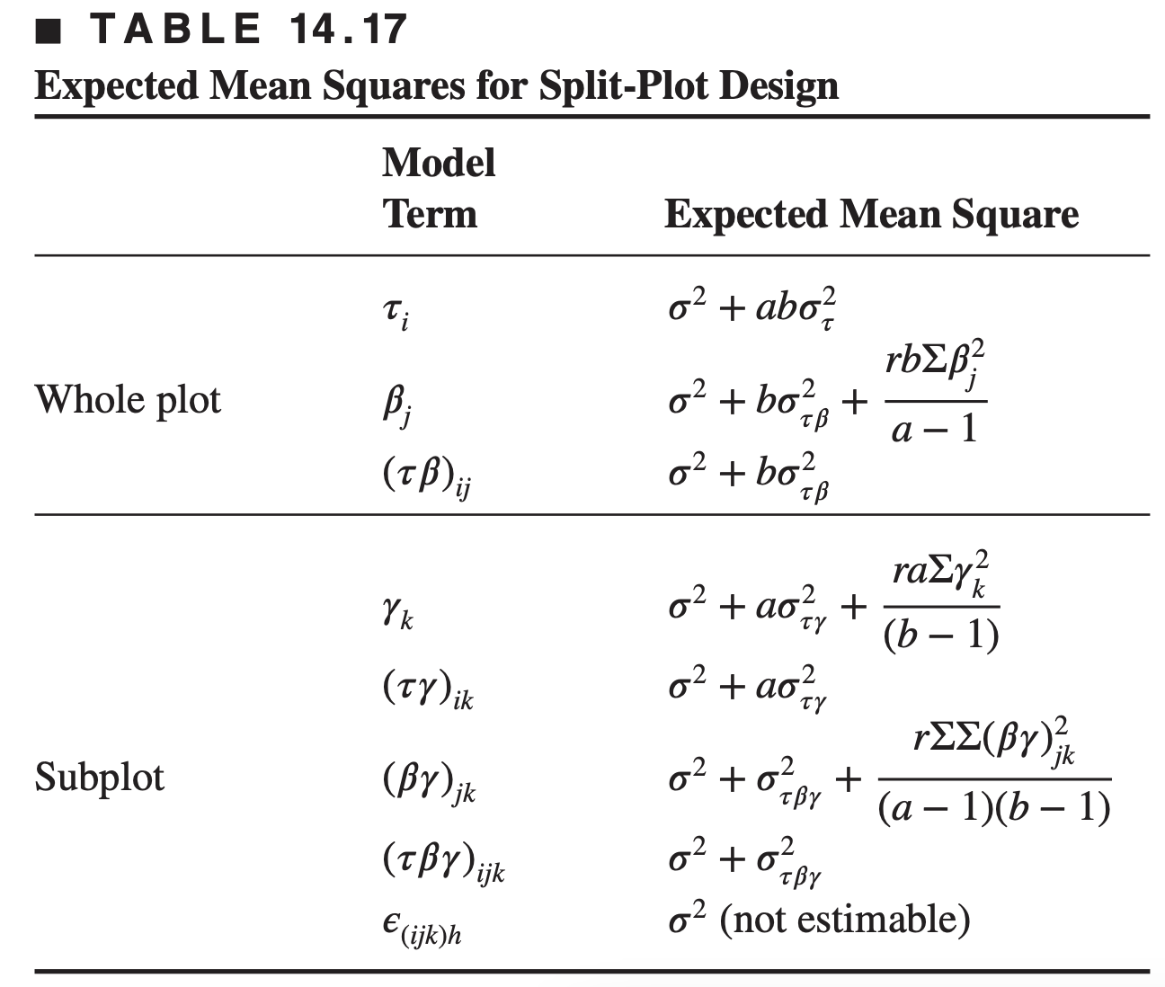
• ${\tau }_i,{\beta }_j$, and $(\tau \beta {)}_{ij}$ represent the whole plot and correspond, respectively, to replicates, main treatments (factor A), and whole-plot error $($ replicates $\times A)$

• ${\gamma }_{\mathrm{k}},(\tau \gamma {)}_{\mathrm{ik}},(\beta \gamma {)}_{\mathrm{jk}}$, and $(\tau \beta \gamma {)}_{\mathrm{ijk}}$ represent the subplot and correspond, respectively, to the subplot treatment (factor $B$ ), the replicates $\times B$ and $AB$ interactions, and the subplot error (replicates $\times$ $\mathrm{AB})$

---

The expected mean squares for the split-plot design, with replicates random and main treatments and subplot treatments fixed, are shown below

---

---

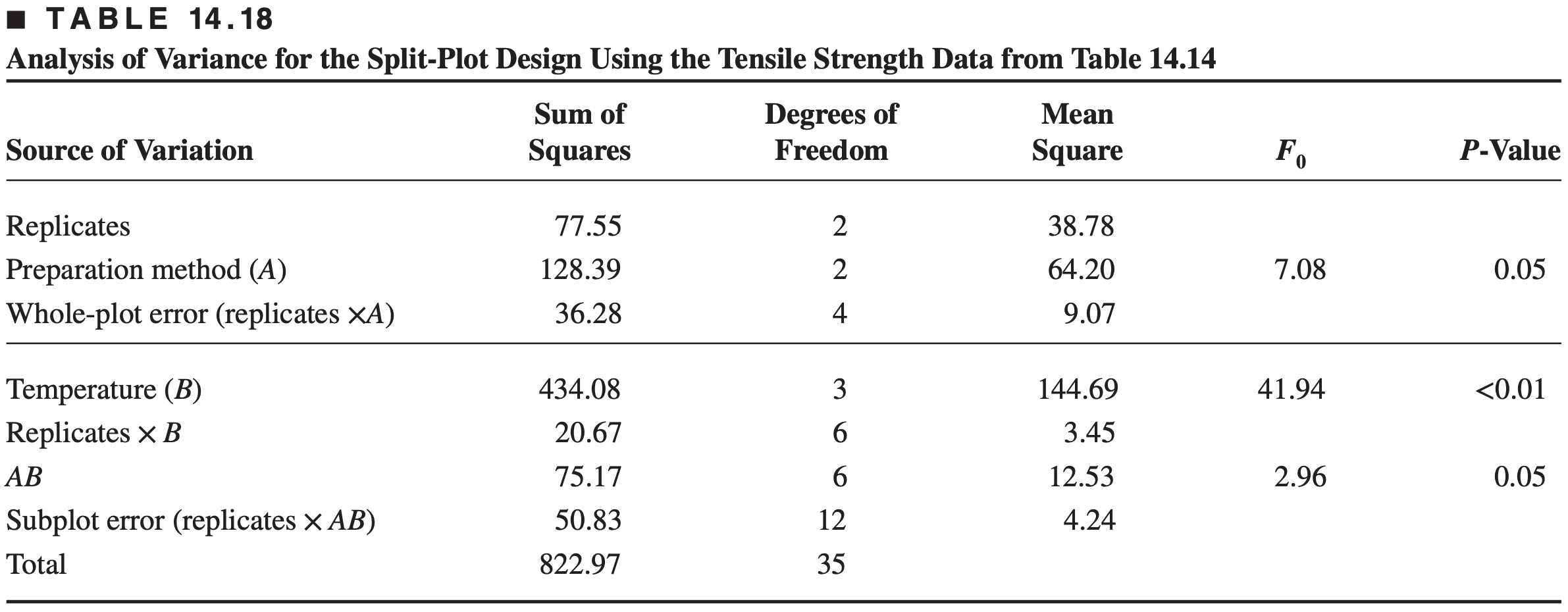
Note from Table 14.18 that the subplot error (4.24) is less than the whole-plot error (9.07).

This is the usual case in split-plot designs because the subplots are generally more homogeneous than the whole plots.

This results in two different error structures for the experiment.

Because the subplot treatments are compared with greater precision, it is preferable to assign the treatment we are most interested in to the subplots, if possible.

---

The split-plot design has an agricultural heritage, with the whole plots usually being large areas of land and the subplots being smaller areas of land within the large areas.

For example, several varieties of a crop could be planted in different fields (whole plots), one variety to a field. Then each field could be divided into, say, four subplots, and each subplot could be treated with a different type of fertilizer.

Here the crop varieties are the main treatments and the different fertilizers are the subtreatments.

---