Chapter 8

(AST301) Design and Analysis of Experiments II

8 Two-Level Fractional Factorial Designs

8.1 Introduction

• As the number of factors in a $2^k$ factorial design increases, the number of runs required for a complete replicate of the design rapidly outgrows the resources of most experimenters.

• For example, a complete replicate of the $2^6$ design requires 64 runs. In this design only 6 of the 63 degrees of freedom correspond to main effects, and only 15 degrees of freedom correspond to two-factor interactions.

• There are only 21 degrees of freedom associated with effects that are likely to be of major interest. The remaining 42 degrees of freedom are associated with three-factor and higher interactions.

---

• If the experimenter can reasonably assume that certain high-order interactions are negligible, information on the main effects and low-order interactions may be obtained by running only a fraction of the complete factorial experiment.

• A major use of fractional factorials is in screening experiments — experiments in which many factors are considered and the objective is to identify those factors (if any) that have large effects.

• The factors identified as important are then investigated more thoroughly in subsequent experiments.

---

Why do Fractional Factorial Designs Work?

The successful use of fractional factorial designs is based on three key ideas:

1. The sparsity of effects principle: when there are several variables, the system will be driven primarily by some of the main effects and low order interactions

2. The projection property: Fractional factorial designs can be projected into larger designs in the subset of significant factors (i.g. Every fractional factorial contains full factorials in fewer factors)

3. Sequential experimentation: It is possible to combine the runs of two or more fractional factorials to assemble sequentially a larger design to estimate the factor effects and interactions of interest

8.2 The one-half fraction of the $2^k$ design

• Consider a situation in which three factors, each at two levels, are of interest, but the experimenters cannot afford to run all $2^3=8$ treatment combinations.

• They can, however, afford four runs.

• This suggests a one-half fraction of a $2^3$ design.

• Because the design contains $2^{3-1}=4$ treatment combinations, a one-half fraction of the $2^3$ design is often called a $2^{3-1}$ design.

---

• The four treatment combinations can be selected according to the plus sign of a factorial effect, which is known as a generator or a word.

• Thus, if $ABC$ is the generator of the $2^{3-1}$ design, then we select the four treatment combinations $a,b,c,$ and $abc$ as our one-half fraction.

• We call $I=ABC$ as the defining relation for the design.

• In general, defining relation will always be the set of all columns that are equal to the identity column $I$.

• The fraction with $I=+ABC$ is called the principal fraction, and $I=-ABC$ is called alternate fraction

---

---

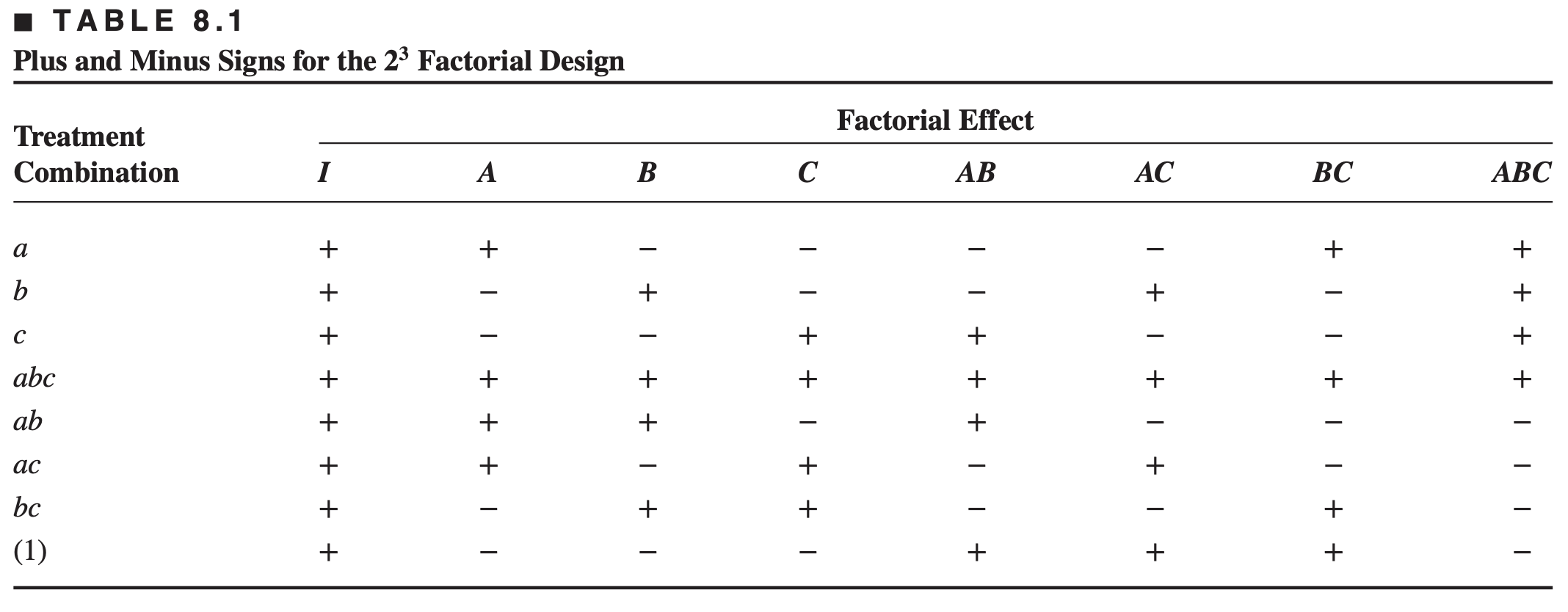
• For the principal fraction, notice that the contrast for $A$ is exactly the same as the contrast for $BC$ interaction

• The estimates of the main effects of $A,B$, and $C$ are $$\begin{array}{rl}& [A]=\frac{1}{2}(a-b-c+abc)\\ & [B]=\frac{1}{2}(-a+b-c+abc)\\ & [C]=\frac{1}{2}(-a-b+c+abc)\end{array}$$

• The estimates of the interactions $AB,BC$, and $AC$ are $$\begin{array}{rl}& [BC]=\frac{1}{2}(a-b-c+abc)\\ & [AC]=\frac{1}{2}(-a+b-c+abc)\\ & [AB]=\frac{1}{2}(-a-b+c+abc)\end{array}$$

---

• Thus, $[A]=[BC],[B]=[AC]$, and $[C]=[AB]$ consequently, it is impossible to differentiate between $A$ and $BC,B$ and $AC$, and $C$ and $AB$.

• In fact, when we estimate $A,B$, and $C$ we are really estimating $A+BC,B+AC$, and $C+AB$. Two or more effects that have this property are called aliases.

• In our example, $A$ and $BC$ are aliases, $B$ and $AC$ are aliases, and $C$ and $AB$ are aliases.

---

• We indicate this by the notation $[A]\to A+BC,[B]$ $\to B+AC$, and $[C]\to C+AB$.

• The alias structure for this design may be easily determined by using the defining relation $I=ABC$.

• Multiplying any column (or effect) by the defining relation yields the aliases for that column (or effect).

• In our example, this yields that the alias of $A$ is $BC$. $$A.I=A.ABC=A^{2}BC=BC$$

• Similarly, we find that ($B$ and $AC$) and ($C$ and $AB$) are aliases

---

• This one-half fraction, with $I=+ABC$, is usually called the principal fraction.

• The other one-half fraction, that is, the treatment combinations associated with minus in the $ABC$ column, known as the complementary or alternate fraction.

• The defining relation for this design is $I=-ABC$.

• The alternate fraction gives us $$\begin{array}{rl}[A{]}^{\prime }& \to A-BC\\ [B{]}^{\prime }& \to B-AC\\ [C{]}^{\prime }& \to C-AB\end{array}$$

---

Thus, when we estimate $A,B$, and $C$ with this particular fraction, we are really estimating $A-BC$, $B-AC$, and $C-AB$.

In practice, it does not matter which fraction is actually used. The two one-half fractions form a complete $2^3$ design.

Suppose that after running one of the one-half fractions of the $2^3$ design, the other fraction was also run. Thus, all eight runs associated with the full $2^3$ are now available.

---

• We may now obtain de-aliased estimates of all the effects by analyzing the eight runs as a full $2^3$ design in two blocks of four runs each.

• This could also be done by adding and subtracting the linear combination of effects from the two individual fractions. $$\begin{array}{rl}& \frac{1}{2}([A]+[A{]}^{\prime })=\frac{1}{2}(A+BC+A-BC)\to A\\ & \frac{1}{2}([A]-[A{]}^{\prime })=\frac{1}{2}(A+BC-A+BC)\to BC\end{array}$$

---

Thus, for all three pairs of linear combinations, we would obtain the following:

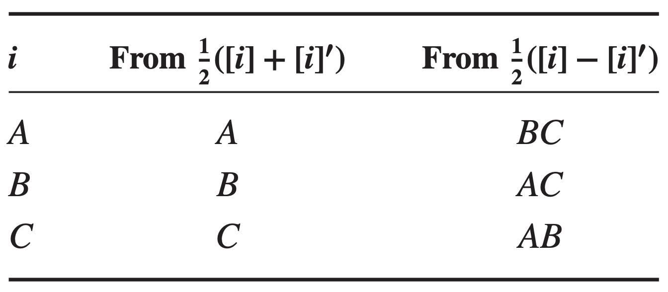
Furthermore, by assembling the full $2^3$ in this fashion with $I=+ABC$ in the first group of runs and $I=-ABC$ in the second, the $2^3$ confounds $ABC$ with blocks

Design resolution

• The preceding $2^3-1$ design is called a resolution III design

• In such a design, main effects are aliased with two-factor interactions.

A design is of resolution $R$ if no $p$-factor effect is aliased with another effect containing less than $R-p$ factors

• We usually employ a Roman numeral subscript to denote design resolution;

• Thus, the one-half fraction of the $2^3$ design with the defining relation $I=ABC$ (or $I=-ABC$) is a $2_{III}^{3-1}$ design.

---

• Design resolutions describe how much the effects in a fractional factorial design are aliased with other effects.

• When we do a fractional factorial design, one or more of the effects are confounded, meaning they cannot be estimated separately from each other.

• Usually, we want to use a fractional factorial design with the highest possible resolution.

---

Resolution III designs.

• These are designs in which no main effects are aliased with any other main effect, but main effects are aliased with two-factor interactions and some two-factor interactions may be aliased with each other.

• The $2^{3-1}$ design in Table 8.1 is of resolution III ($2_{III}^{3-1}$)

---

Resolution IV design.

• These are designs in which no main effect is aliased with any other main effect or with any two-factor interaction, but two-factor interactions are aliased with each other.

• A $2^{4-1}$ design with $I=ABCD$ is a resolution $IV$ design ($2_{IV}^{4-1}$)

---

Resolution V design.

• These are designs in which no main effect or two-factor interaction is aliased with any other main effect or two-factor interaction, but two-factor interactions are aliased with three-factor interactions.

• A $2^{5-1}$ design with $I=ABCDE$ is a resolution $V$ design ($2_V^{5-1}$)

---

• In general, the resolution of a two-level fractional factorial design is equal to the shortest number of letters in any word in the defining relation

Higher the resolution better the design (why?)

---

• We never want a resolution II design, because a design would alias two main effects. Thus minimum acceptable resolution in III.

• Resolution III designs have some main effects aliased to two-factor interactions. If we believe that only main effects are present and all interactions are negligible, then a resolution III design is sufficient for estimating main effects.

• Resolution III designs are called main effects design for this reason.

• If we believe that some two factor interactions may be non negligible but all three way and higher interactions are negligible then a resolution IV is sufficient for main effects.

• Low resolution fractional factorials are often used as screening designs, where we are trying to screen many factors to see if any of them has an effect. This is usually an early stage of investigation.

Construction and Analysis of the One-Half Fraction

A one-half fraction of the $2^k$ design of the highest resolution may be constructed by

• writing down a basic design consisting of the runs for a full $2^{k-1}$ factorial and

• then adding the the $k^{\text{th}}$ factor by identifying its plus and minus levels with the plus and minus signs of the highest order interaction $ABC\cdots (K-1)$

Constructing one-half fractions

• E.g. the $2_{III}^{3-1}$ fractional factorial design of the highest resolution can be obtained by writing down the full $2^2$ factorial as the basic design and then equating the factor $C$ to $AB$

---

• Note that any interaction effect could be used to generate the column for the $k$th factor.

• However, using any effect other than $ABC$….(K-1) will not produce a design of the highest possible resolution.

• Another way to view the construction of a one-half fraction is to partition the runs into two blocks with the highest order interaction $ABC\dots K$ confounded. Each block is a $2^{k-1}$ fractional factorial design of the highest resolution.

---

Sequences of fractional factorials

• Fractional factorial designs could be less expensive and efficient in experimentation, if the runs can be made sequentially

• If the interest is in investigating $k=4$ factors (i.e. $2^4=16$ runs) then it is preferable to run a $2_{IV}^{4-1}$ fractional design, analyze the results, and then decide on the best set of runs to perform the next.

• If necessary we can always run the alternate fraction and get the complete $2^4$ design, where both half-fractions are considered as blocks

---

Projection of Fractions into Factorials

Any fractional factorial design of resolution $R$ contains complete factorial designs (possibly replicated factorials) in any subset of $R-1$ factors.

• This is an important and useful concept

• Because the maximum possible resolution of a one-half fraction of the $2^k$ design is $R=k$, every $2^{k-1}$ design will project into a full factorial in any ($k-1$) of the original $k$ factors.

• Furthermore, a $2^{k-1}$ design may be projected into two replicates of a full factorial in any subset of $k-2$ factors, four replicates of a full factorial in any subset of $k-3$ factors, and so on.

EXAMPLE 8.1

• Consider the filtration rate experiment in Example 6.2. The original design is a single replicate of the $2^4$ design.

• In that example, we found that the main effects $A$, $C$, and $D$ and the interactions $AC$ and $AD$ were different from zero.

• We will now return to this experiment and simulate what would have happened if a half-fraction of the $2^4$ design had been run instead of the full factorial.

---

---

---

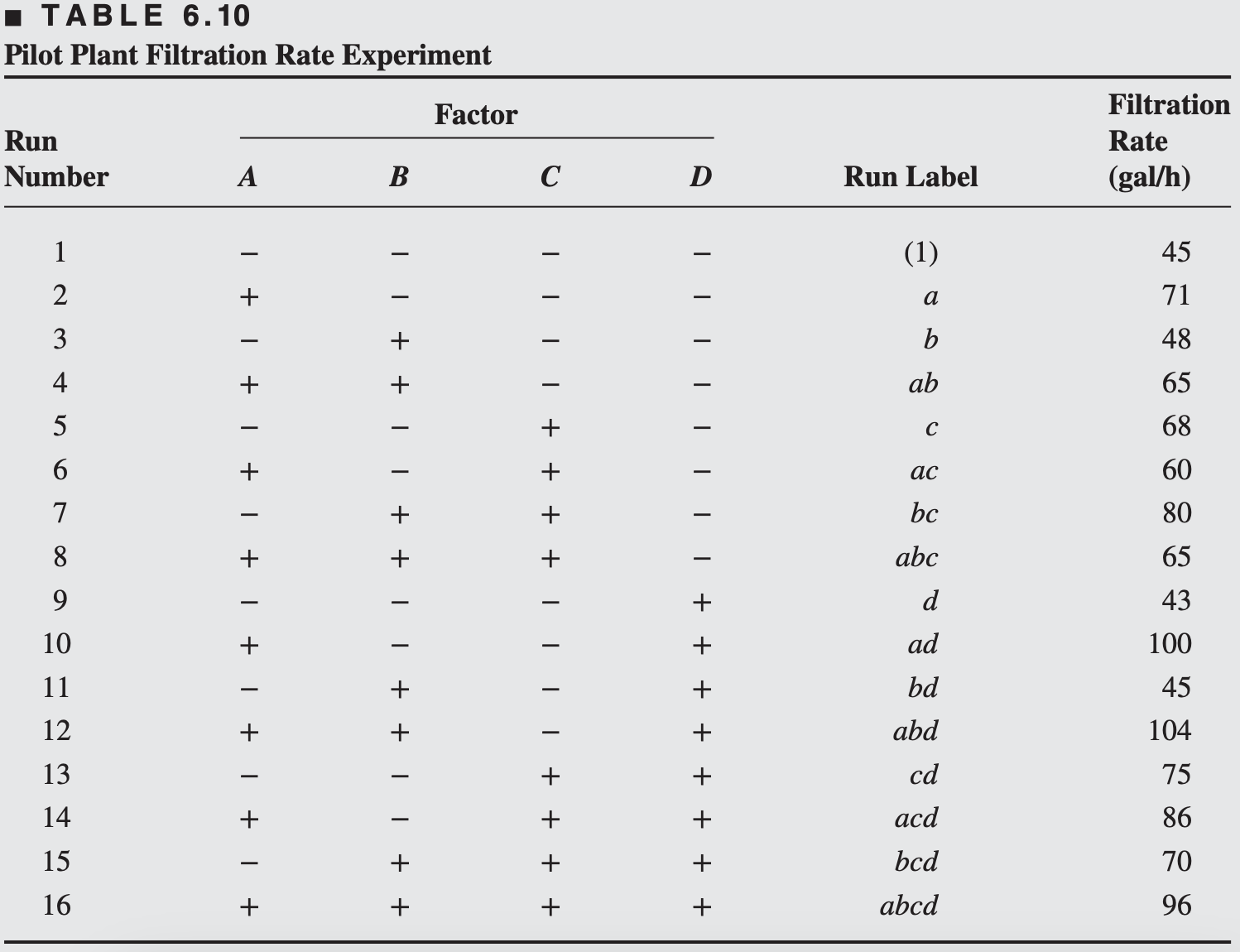
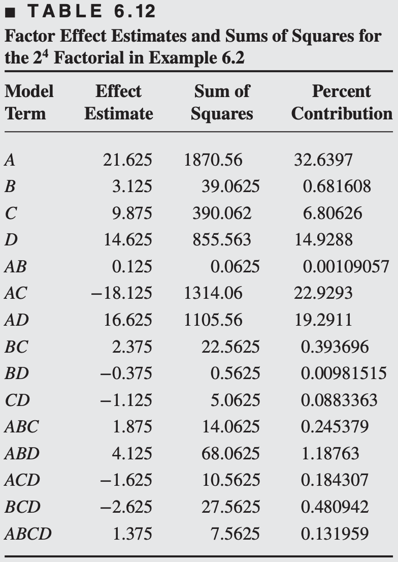
We will use the $2^{4-1}$ design with $I=ABCD$.

---

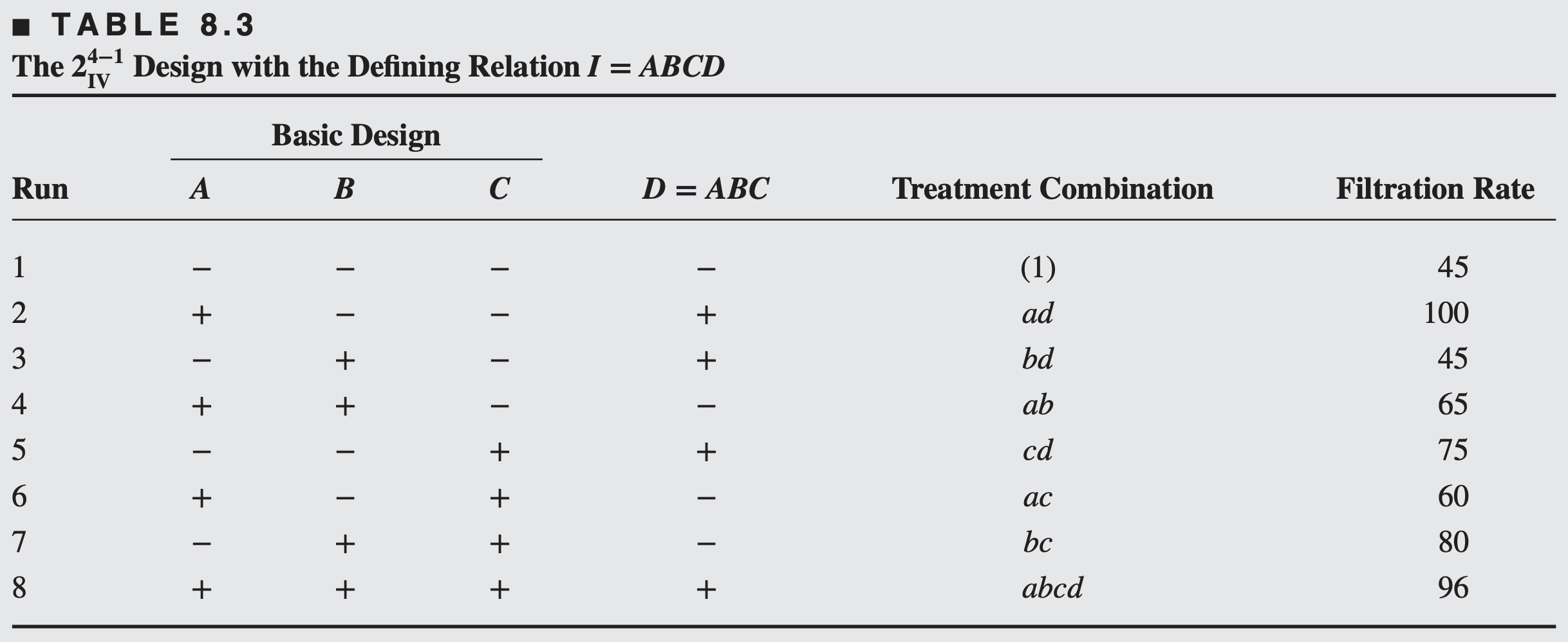
• Using the defining relation, we note that each main effect is aliased with a three-factor interaction; that is, $A=A^{2}BCD=BCD,B={AB}^{2}CD=ACD,C={ABC}^{2}D=$ $ABD$, and $D={ABCD}^2=ABC$.

• Furthermore, every two-factor interaction is aliased with another two-factor interaction. These alias relationships are $AB=CD,AC=BD$, and $BC=AD$.

• The four main effects plus the three two-factor interaction alias pairs account for the seven degrees of freedom for the design.

---

$\begin{array}{rl}[A]=& \frac{1}{4}(-45+100-45+65-75\\ & +60-80+96)=19.00\to A+BCD\\ [AB]=& \frac{1}{4}(45-100-45+65+75-60-80+96)\\ =& -1.00\to AB+CD\end{array}$

---

---

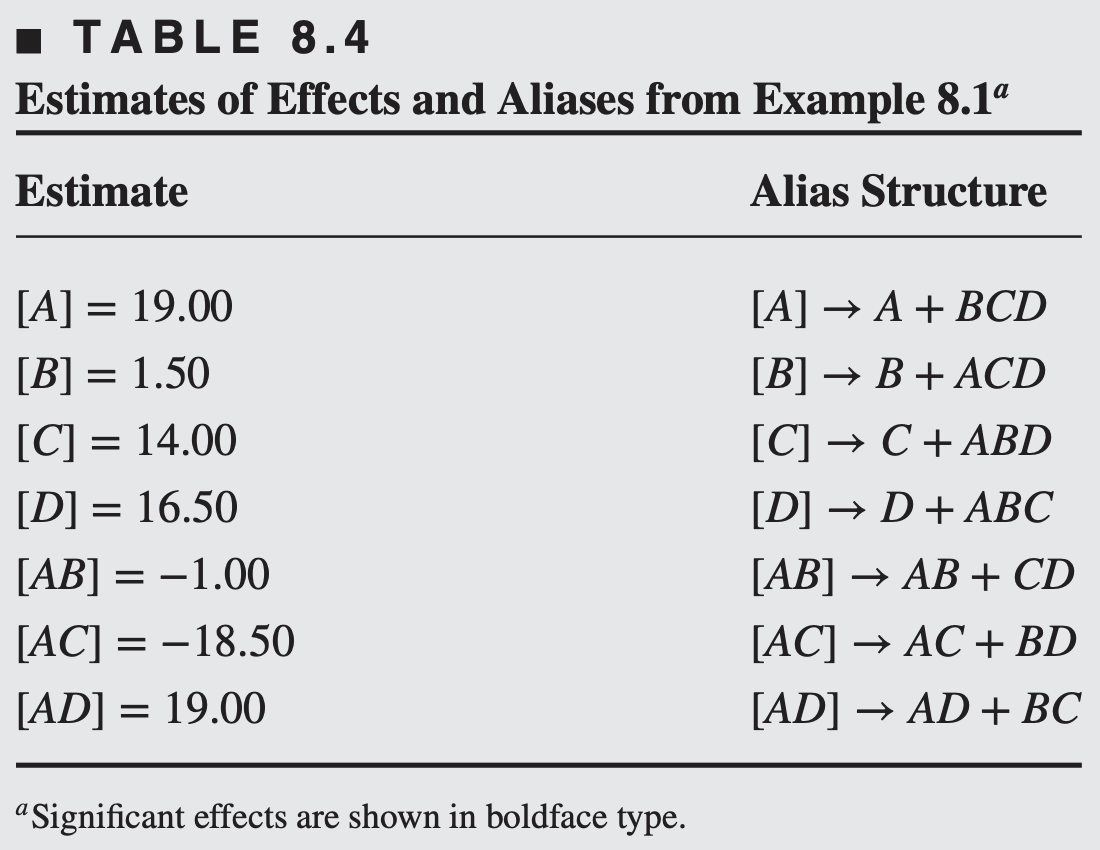
• Because factor B is not significant, we may drop it from consideration. Consequently, we may project this design into a single replicate of the $2^3$ design in factors $A,C$, and $D$.

• Based on the above analysis, we can now obtain a model to predict filtration rate over the experimental region. This model is

$\begin{array}{rl}\hat{y}=& {\hat{\beta }}_0+{\hat{\beta }}_1{x}_1+{\hat{\beta }}_3{x}_3+{\hat{\beta }}_4{x}_4+{\hat{\beta }}_{13}{x}_1{x}_3+{\hat{\beta }}_{14}{x}_1{x}_4\\ \hat{y}=& 70.75+\left(\frac{19.00}{2}\right)x_1+\left(\frac{14.00}{2}\right)x_3+\left(\frac{16.50}{2}\right)x_4\\ & +\left(\frac{-18.50}{2}\right)x_1{x}_3+\left(\frac{19.00}{2}\right)x_1{x}_4\end{array}$

---

• There are two large effects associated with two-factor interactions, $AC+BD$ and $AD+BC$.

• In Example $8.2$, we used the fact that the main effect of $B$ was negligible to tentatively conclude that the important interactions were $AC$ and $AD$.

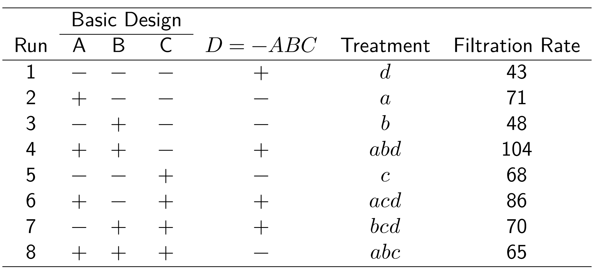
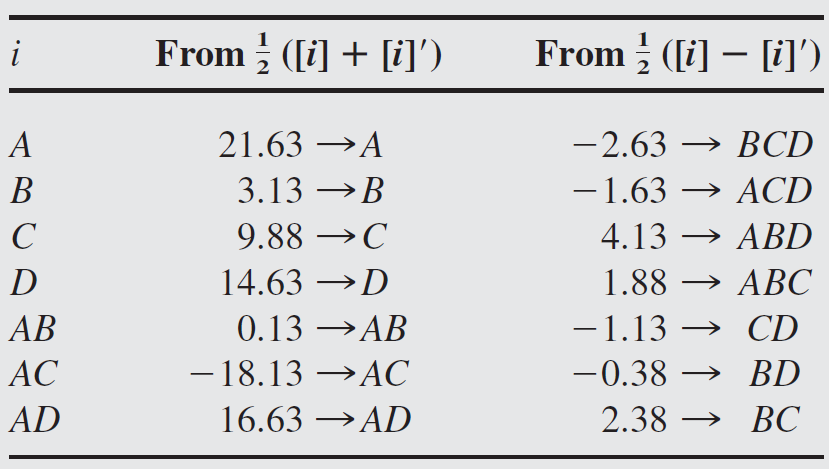
• However, we can always isolate the significant interaction by running the alternate fraction, given by $I=-ABCD$.

---

---

---

8.3 The one-quarter fraction of the $2^k$ design

• One-quarter fraction of the $2^k$ design could be useful when the number of factors is large.

• This design contains $2^{k-2}$ runs and is usually called a $2^{k-2}$ fractional factorial.

• The construction of the $2^{k-2}$ fractional factorial design requires to write down the basic design with $k-2$ factors first and then two additional columns are constructed from appropriately chosen interactions involving the first $k-2$ factors.

---

• The one-quarter fraction of the $2^k$ design has two generators, if $P$ and $Q$ are the two generators then their generalized interaction $PQ$ also acts as a generator

• Complete defining relation is $I=P=Q=PQ$

• As an example, consider $2^{6-2}$ design with $I=ABCE$ and $I=BCDF$ as the design generators

  • The complete defining relation for this design is $I=ABCE=BCDF=ADEF(ABCE\times BCDF)$

  • This $2^{6-2}$ design is a resolution $IV$ design, why?

---

• For the $2^{6-2}$ design with $I=ABCE=BCDF=ADEF$, the main effects are aliased with two- and five-factor interactions, e.g.
  $$\begin{array}{rl}A(I)& =A(ABCE)=A(BCDF)=A(ADEF)\\ A& =BCE=ABCDF=DEF\end{array}$$

• When we estimate the main effect of $A$, we actually estimate $A+BCE+DEF+ABCDF$

• Similarly, when we estimate 2-factor interaction $AB$, we actually estimate $AB+CE+ACDF+BDEF$

---

The complete alias structure of this design is

---

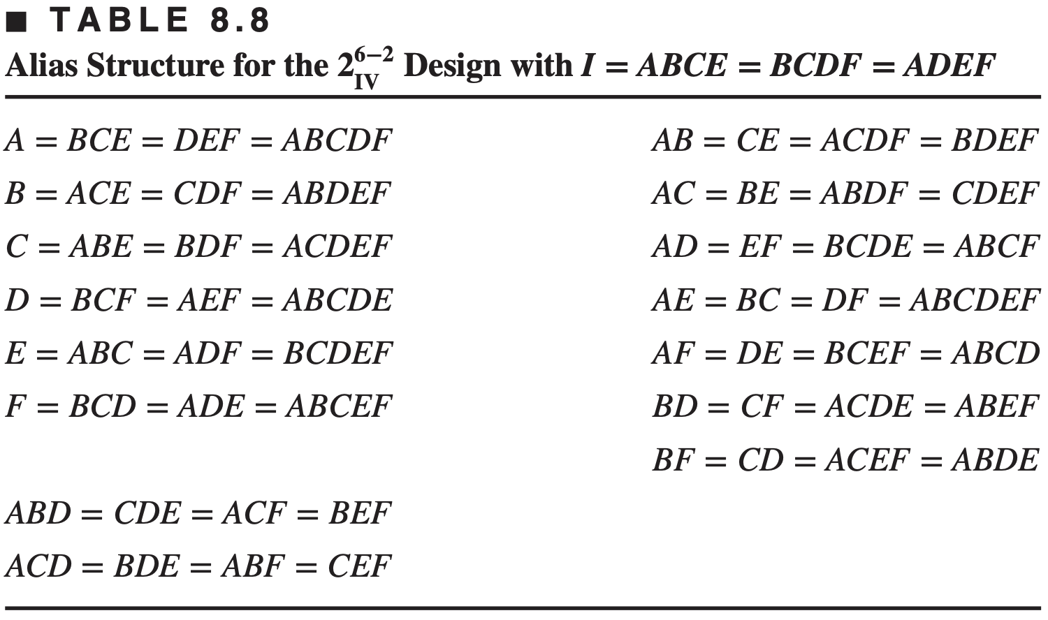
• To construct the design, first write down the basic design, which consists of the 16 runs for a full $2^{6-2}$ $=2^4$ design in $A,B,C$, and $D$.

• Then the two factors $E$ and $F$ are added by associating their plus and minus levels with the plus and minus signs of the interactions $ABC$ and $BCD$, respectively. This procedure is shown below

---

---

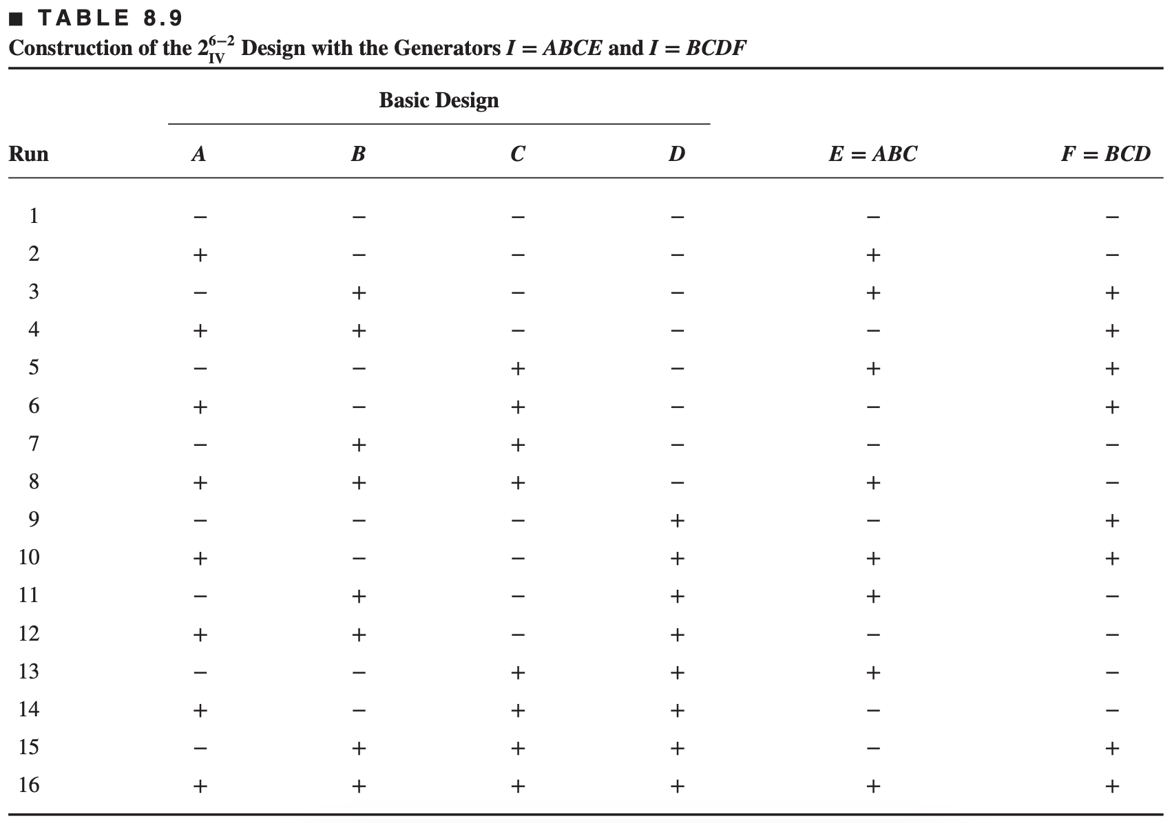
• Another way to construct this design is to derive the four blocks of the $2^6$ design with $ABCE$ and $BCDF$ confounded and then choose the block with treatment combinations that are positive on $ABCE$ and $BCDF$.

• This would be a $2^{6-2}$ fractional factorial with generating relations $I=ABCE$ and $I=BCDF$, and because both generators $ABCE$ and $BCDF$ are positive, this is the principal fraction.

---

• For this $2^{6-2}$ design, there are three alternate fractions, which are $$\begin{array}{rl}I& =ABCE,I=-BCDF;\\ I& =-ABCE,I=BCDF;\text{and}\\ I& =-ABCE,I=-BCDF\end{array}$$

EXAMPLE 8.4

A quality improvement team has decided to use a designed experiment to study the injection molding process so that shrinkage can be reduced. The team decides to investigate six factors Mold temperature ($A$), Screw speed ($B$), Holding time ($C$), Cycle time ($D$), Gate size ($E$), and holding pressure ($F$) - each at two levels.

The objective of this experiment is of learning how each factor affects shrinkage and also, something about how the factors interact. The team decides to use the 16-run two-level fractional factorial design.

---

---

---

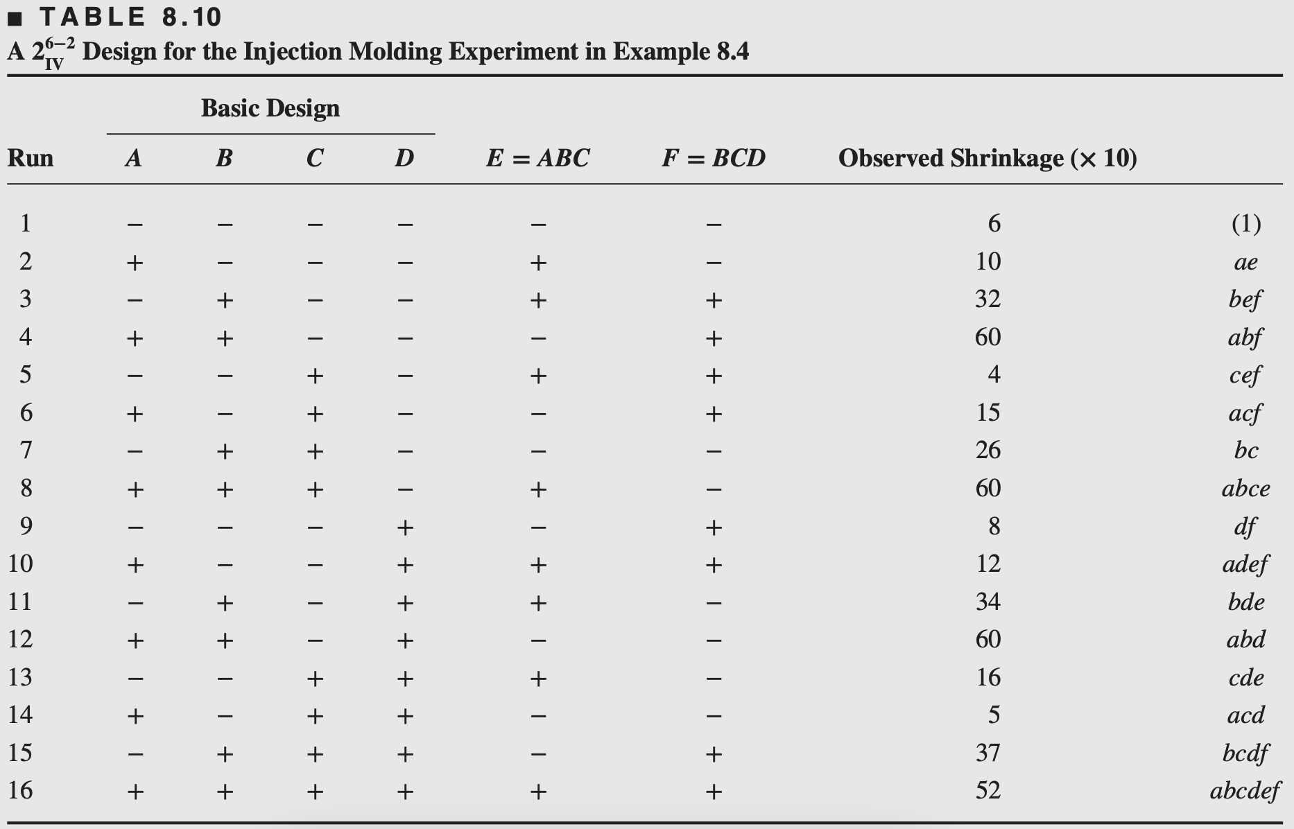
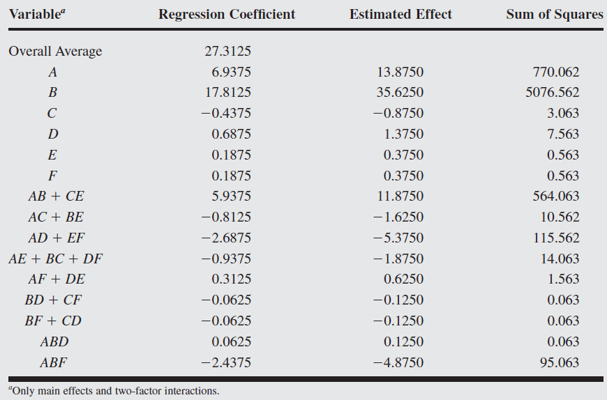
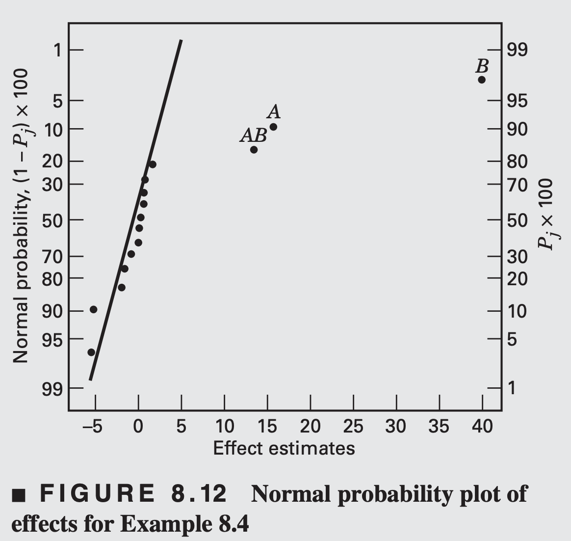
The only large effects are A (mold temperature), B (screw speed), and the AB interaction

---

---

---

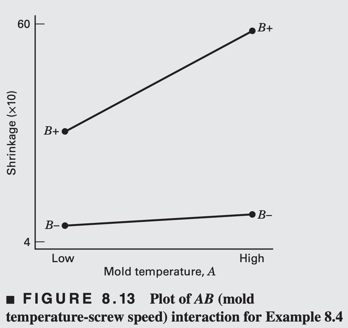
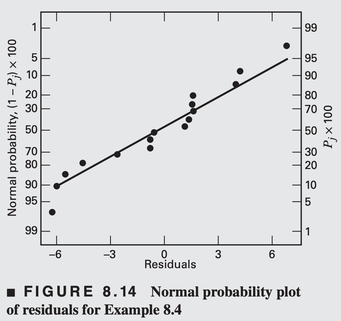
• The plot of the AB interaction shows that the process is very insensitive to temperature if the screw speed is at the low level but very sensitive to temperature if the screw speed is at the high level.

• Based on this initial analysis, the team decides to set both the mold temperature and the screw speed at the low level

8.4 The general $2^{k-p}$ fractional factorial design

• A $2^k$ fractional design containing $2^{k-p}$ runs is called $1/2^p$ fraction of the $2^k$ design or $2^{k-p}$ fractional factorial design

• These designs require the selection of $p$ independent generators and the corresponding defining relation consists of the initially chosen $p$ generators and their $2^p-p-1$ generalized interactions

• The alias structure can be found by multiplying each effect column by the defining relation and generators should be chosen carefully so that effects of potential interest are not aliased with each other, and each effect will have $2^p-1$ aliases

• For moderately large values of $k$, we usually assume higher order interactions (say, third- or fourth-order and higher) to be negligible, and this greatly simplifies the alias structure.

---

• It is important to select the $p$ generators for a $2^{k-p}$ fractional factorial design in a way that we obtain the best possible alias relationships

• A reasonable criterion is to select the generators such that the resulting $2^{k-p}$ design has the highest possible resolution, e.g. consider a $2^{6-2}$ design

Defining relation $I=ABCE=ABCDF\to$ Resolution III

Defining relation $I=ABCE=BCDF\to$ Resolution IV

---

• Sometimes resolution alone is insufficient to distinguish between designs. For example, consider the three $2{}_{IV}{}^{7-2}$ designs, which are based on different defining relations, but have the equal resolution $IV$.

• Sometimes resolution alone is insufficient to distinguish between designs. consider the three $2{}_{IV}{}^{7-2}$ designs given below

---

---

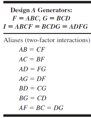
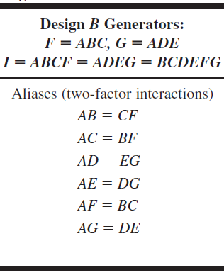
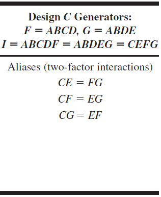
• All of these designs are of resolution IV, but they have rather different alias structures (we have assumed that three-factor and higher interactions are negligible) with respect to the two-factor interactions.

• Clearly, design A has more extensive aliasing and design $C$ the least, so design $C$ would be the best choice for a $2_{IV}{}^{7-2}$.

• The three word lengths in design A are all 4; that is, the word length pattern is $\{4,4,4\}$.

---

• For design $B$ it is $\{4,4,6\}$, and for design $C$ it is $\{4,5,5\}$

• Notice that the defining relation for design $C$ has only one four-letter word, whereas the other designs have two or three.

• Thus, design $C$ minimizes the number of words in the defining relation that are of minimum length. We call such a design a minimum aberration design.

---

Minimizing aberration in a design of resolution $R$ ensures that the design has the minimum number of main effects aliased with interactions of order $R-1$, the minimum number of two-factor interactions aliased with interactions of order $R-2$, and so forth.

Table $8.14$ presents a selection of $2^{k-p}$ fractional factorial designs for $k\le 15$ factors and up to $n\le 128$ runs.

The suggested generators in this table will result in a design of the highest possible resolution. These are also the minimum aberration designs.

---

---

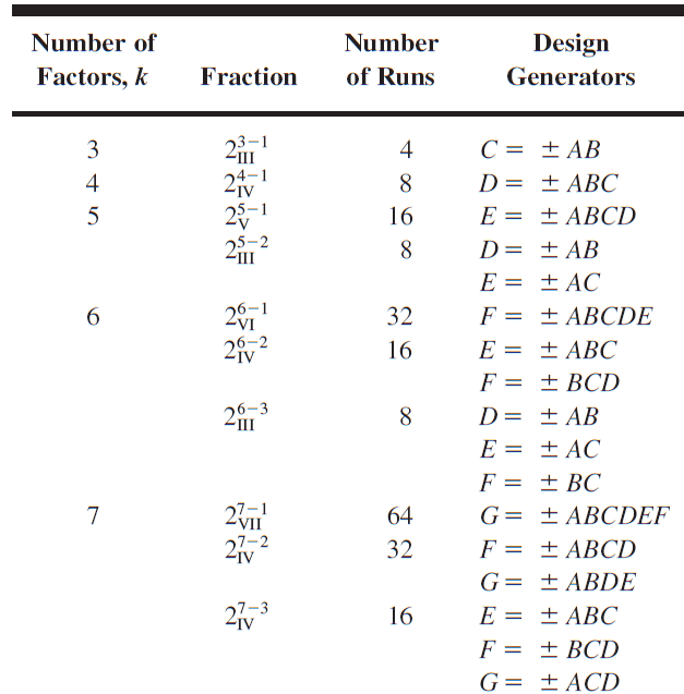
The alias relationships for all of the designs in Table $8.14$ for which $n\le 64$ are given in Appendix Table X(a-w).

The alias relationships presented in this table focus on main effects and two- and three-factor interactions. The complete defining relation is given for each design.

This appendix table makes it very easy to select a design of sufficient resolution to ensure that any interactions of potential interest can be estimated.

Analysis of $2^{k-p}$ fractional factorials

• The $i^{\text{th}}$ effect is estimated by $$\begin{array}{rl}{l}_i& =\frac{{\text{contrast}}_i}{(N/2)},\end{array}$$ where ${\text{contrast}}_i$ can be found from the plus and minus sign of the column $i$ and $N=2^{k-p}$ is the total number of observations

• The $2^{k-p}$ design allows only $2^{k-p}-1$ effects (and their aliases) to be estimated

Exercise 8.12.

An article in Industrial and Engineering Chemistry (“More on Planning Experiments to Increase Research Efficiency,” 1970, pp. 60-65) uses a $2^{5-2}$ design to investigate the effect of $A=$ condensation temperature, $B=$ amount of material $1,C=$ solvent volume, $D=$ condensation time, and $E=$ amount of material 2 on yield. The results obtained are as Follows:

$$\begin{array}{rl}& e=23.2ad=16.9cd=23.8bde=16.8\\ & ab=15.5bc=16.2ace=23.4\text{ abcde }=18.1\end{array}$$

1. Verify that the design generators used were I $=ACE$ and $I=BDE$.

2. Write down the complete defining relation and the aliases for this design.

3. Estimate the main effects.

---

4. Prepare an analysis of variance table. Verify that the AB and AD interactions are available to use as error.

5. Plot the residuals versus the fitted values. Comment on the results.

8.4.3 Blocking Fractional Factorials

• Occasionally, a fractional factorial design requires so many runs that all of them cannot be made under homogeneous conditions.

• In these situations, fractional factorials may be confounded in blocks.

• Appendix Table X contains recommended blocking arrangements for many of the fractional factorial designs in Table 8.14. The minimum block size for these designs is eight runs

---

• In assigning fractional factorials into blocks, we need to be careful about the effects to be confounded with blocks

• The $2_{IV}^{6-2}$ design with $I=ABCE=BCDF=ADEF$ is $$\begin{array}{r}(1),df,cef,bef,a,abef,acf,bc,\\ adef,bde,cde,abce,abd,acd,bcdf,abcdef,\end{array}$$

• This fractional design contains 16 treatment combinations.

• We want to conduct the experiment into two blocks. Which effect should we select to be confounded with blocks?

---

• In selecting an interaction to confound with blocks, we note from examining the alias structure in Appendix Table IX(f) that there are two alias sets involving only three-factor interactions.

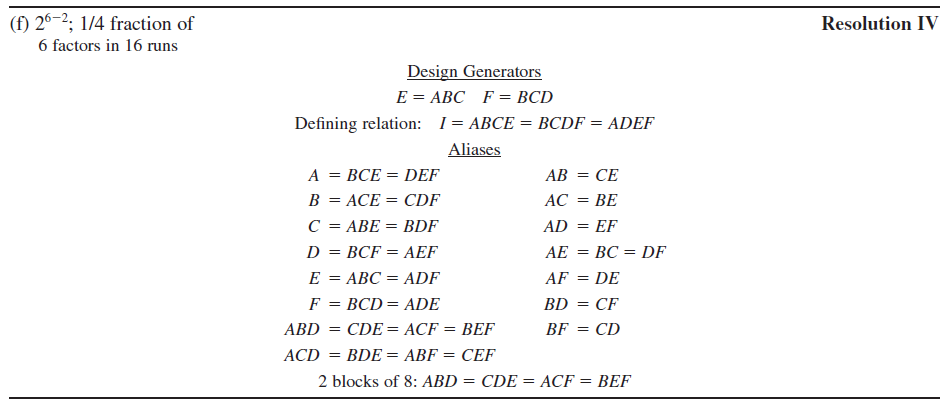
• The table suggests selecting ABD (and its aliases) to be confounded with blocks.

---

• Assume the effect $ABD$ confounded with blocks, so the defining contrast $L=x_1+x_2+x_4=0(\text{mod}2)$

$$\begin{array}{r}(1),df,cef,bef,a,abef,acf,bc,\\ adef,bde,cde,abce,abd,acd,bcdf,abcdef,\end{array}$$

Block-1 $(L=0)$ $$\begin{array}{r}(1),abef,adef,bde\\ abce,acd,bcdf,abcdef\end{array}$$

Block-2 $(L=1)$ $$\begin{array}{r}df,cef,bef,a,acf,\\ bc,cde,abd\end{array}$$

• Notice that the principal block contains those treatment combinations that have an even number of letters in common with ABD.

Example 8.6

A five-axis CNC machine is used to produce an impeller for a jet turbine engine. The blade profiles are an important quality characteristic.

Specifically, the deviation of the blade profile from the profile specified on the engineering drawing is of interest.

An experiment is run to determine which machine parameters affect profile deviation.

---

The eight factors selected for the design are as follows: $$\begin{array}{rl}& A=\text{ x-Axis shift}\\ & B=\text{ y-Axis shift }\\ & C=\text{ z-Axis shift }\\ & D=\text{ Tool supplier }\\ & E=\text{ a-Axis shift }\\ & F=\text{ Spindle speed }(\mathrm{\%})\\ & G=\text{ Fixture height }\\ & H=\text{ Feed rate }(\mathrm{\%})\end{array}$$

---

The profile deviation is measured using a coordinate measuring machine, and the standard deviation of the difference between the actual profile and the specified profile is used as the response variable.

The machine has four spindles. Because there may be differences in the spindles, the process engineers feel that the spindles should be treated as blocks.

---

The engineers feel confident that three-factor and higher interactions are not too important, but they are reluctant to ignore the two-factor interactions.

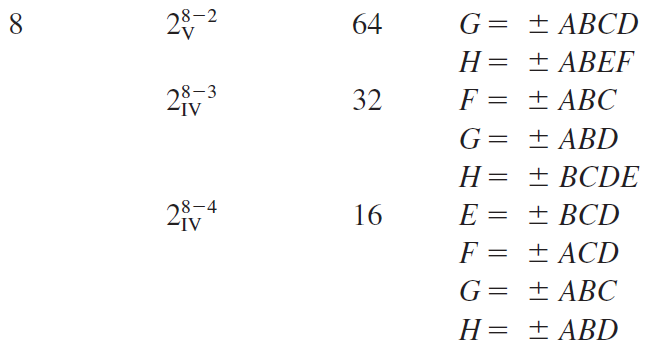
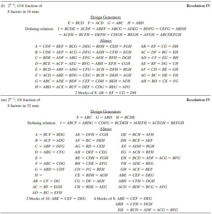
From Table 8.14, two designs initially appear appropriate: the $2_{IV}^{8-4}$ design with 16 runs and the $2_{IV}^{8-3}$ design with 32 runs. The experimenters decide to use the $2_{IV}^{8-3}$ design in four blocks.

---

---

---

---

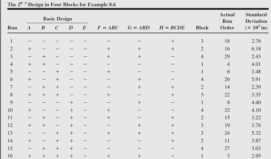
Because the response variable is a standard deviation, it is often best to perform the analysis following a log transformation.

---

---

---

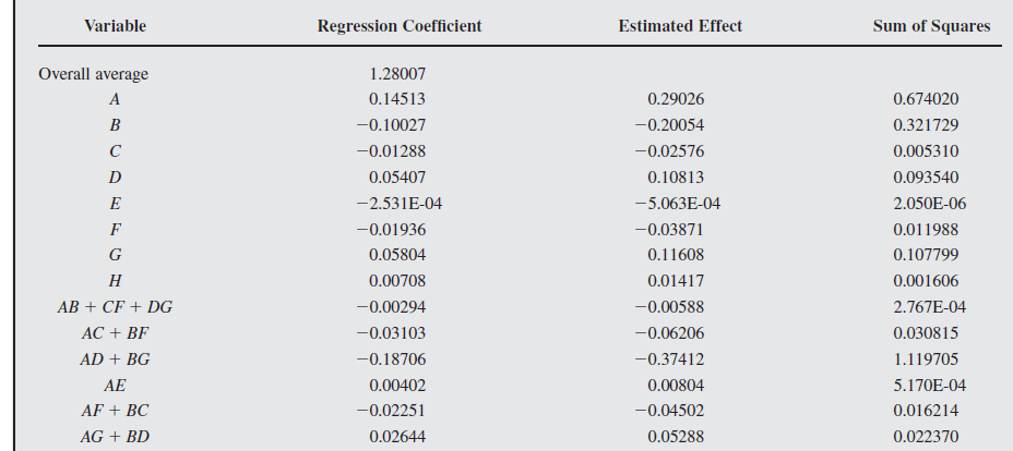
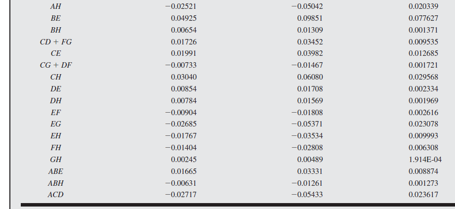
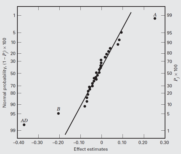
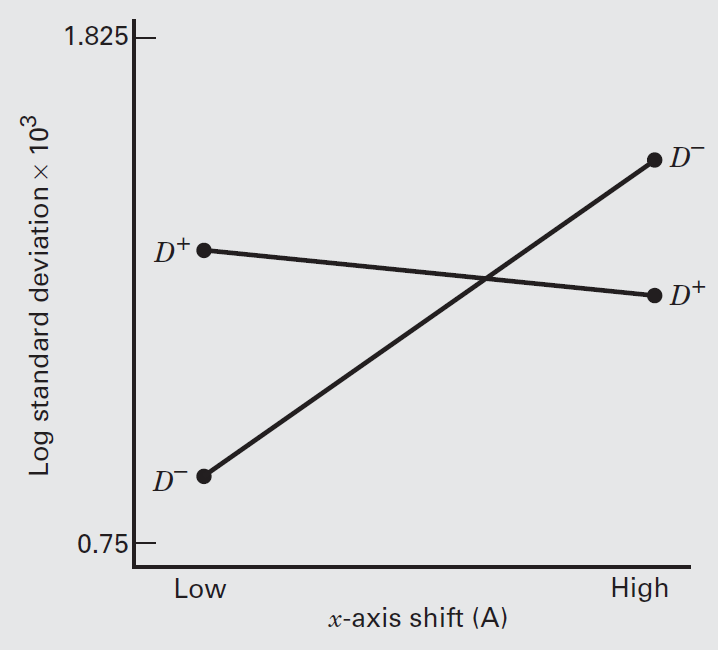
Suppose that process knowledge suggests that the appropriate interaction is likely to be $AD$.

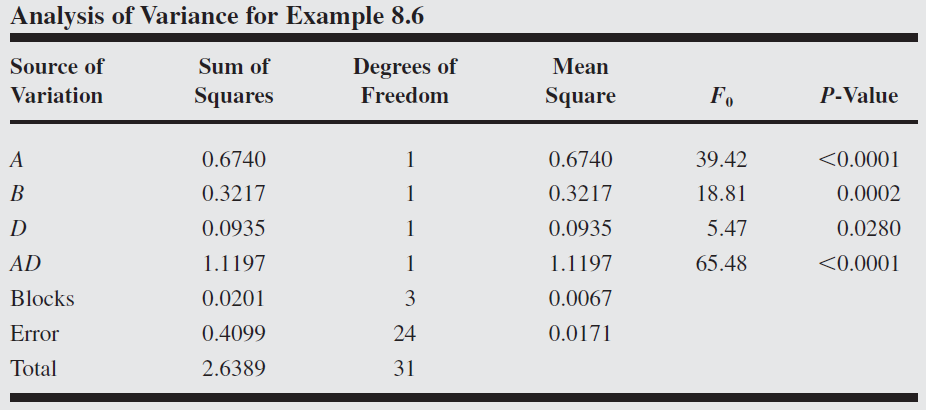
Following table shows the resulting analysis of variance for the model with factors $A$, $B$, $D$, and $AD$ (factor $D$ was included to preserve the hierarchy principle).

Notice that the block effect is small, suggesting that the machine spindles are not very different.

---

---

---

---

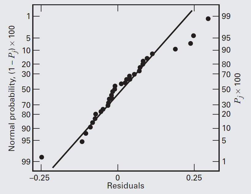
Normal probability plot of the residuals is suggestive of slightly heavier than normal tails, so possibly other transformations should be considered.

The $AD$ interaction plot shows that running $A$ at the low level ( 0 offset) and buying tools from supplier 1 gives the best results.

The projection of this design into four replicates of a $2^3$ design in factors $A,B$, and $D$ is shown below.

---

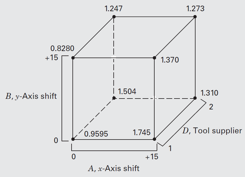
The figure indicates that the best combination of operating conditions is $A$ at the low level (0 offset), $B$ at the high level (0.015 in offset), and $D$ at the low level (tool supplier 1).

Exercise 8.45

Consider the design:

---

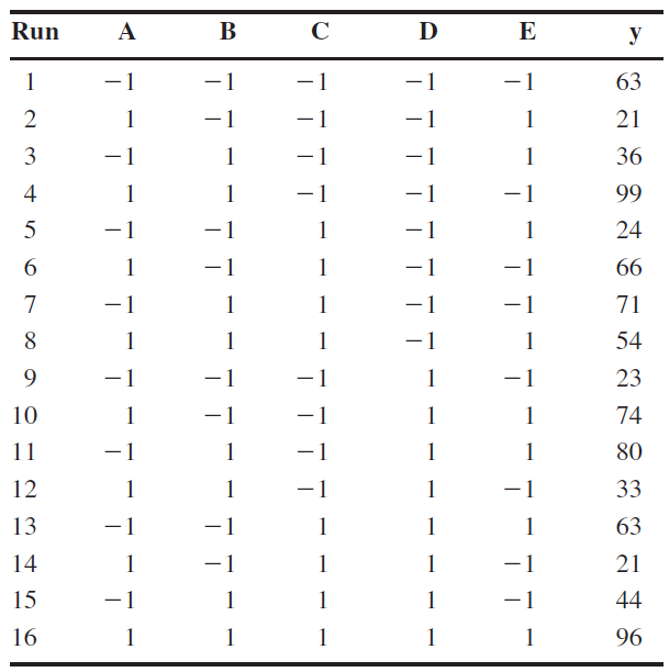
1. What is the generator for column $E$?
2. If $ABC$ is confounded with blocks, run 1 above goes in the —- block. Answer either $+$ or $-$.
3. What is the resolution of this design?
4. Find the estimates of the main effects and their aliases.

8.5 Alias Structures in Fractional Factorials and Other Designs

Alias Structures in General Fractionals

In this chapter, we show how to find the alias relationships in a $2^{k-p}$ fractional factorial design by use of the complete defining relation.

This method works well in simple designs, such as the regular fractions we use most frequently, but it does not work as well in more complex settings, such as some of the nonregular fractions and partial fold-over designs that we will discuss subsequently.

Furthermore, there are some fractional factorials that do not have defining relations, such as the Plackett-Burman designs in Section 8.6.3, so the defining relation method will not work for these types of designs at all.

Fortunately, there is a general method available that works satisfactorily in many situations.

---

The method uses the polynomial or regression model representation of the model, say $$\mathbf{y}={\mathbf{X}}_1{\mathit{\beta }}_1+\mathit{ϵ}$$ where $\mathbf{y}$ is an $n\times 1$ vector of the responses, ${\mathbf{X}}_1$ is an $n\times p_1$ matrix containing the design matrix expanded to the form of the model that the experimenter is fitting, ${\mathit{\beta }}_1$ is a $p_1\times 1$ vector of the model parameters, and $ϵ$ is an $n\times 1$ vector of errors.

The least squares estimate of ${\mathit{\beta }}_1$ is $${\hat{\mathit{\beta }}}_1={\left({\mathbf{X}}_1^{\prime }{\mathbf{X}}_1\right)}^{-1}{\mathbf{X}}_1^{\prime }\mathbf{y}$$

---

Suppose that the true model is $$\mathbf{y}={\mathbf{X}}_1{\mathit{\beta }}_1+{\mathbf{X}}_2{\mathit{\beta }}_2+ϵ$$ where ${\mathbf{X}}_2$ is an $n\times p_2$ matrix containing additional variables that are not in the fitted model and ${\mathit{\beta }}_2$ is a $p_2\times 1$ vector of the parameters associated with these variables.

It can be shown that $$\begin{array}{rl}E\left({\hat{\mathit{\beta }}}_1\right)& ={\mathit{\beta }}_1+{\left({\mathbf{X}}_1^{\prime }{\mathbf{X}}_1\right)}^{-1}{\mathbf{X}}_1^{\prime }{\mathbf{X}}_2{\mathit{\beta }}_2\\ & ={\mathit{\beta }}_1+\mathbf{A}{\mathit{\beta }}_2\end{array}$$

The matrix $\mathbf{A}={\left({\mathbf{X}}_1^{\prime }{\mathbf{X}}_1\right)}^{-1}{\mathbf{X}}_1^{\prime }{\mathbf{X}}_2$ is called the alias matrix.

---

The elements of this matrix operating on ${\mathit{\beta }}_2$ identify the alias relationships for the parameters in the vector ${\mathit{\beta }}_1$.

We illustrate the application of this procedure with a familiar example. Suppose that we have conducted a $2^{3-1}$ design with defining relation $I=ABC$ or $I=x_1{x}_2{x}_3$. The model that the experimenter plans to fit is the main-effects-only model $$y={\beta }_0+{\beta }_1{x}_1+{\beta }_2{x}_2+{\beta }_3{x}_3+ϵ$$

---

---

---

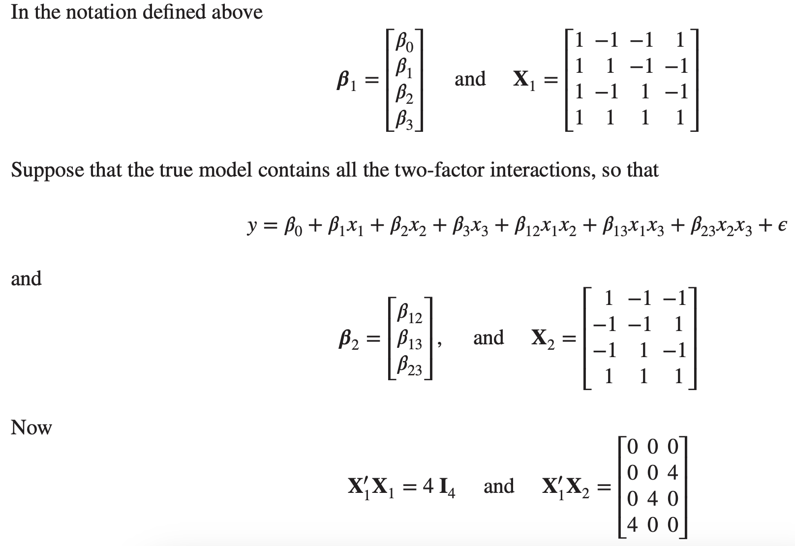
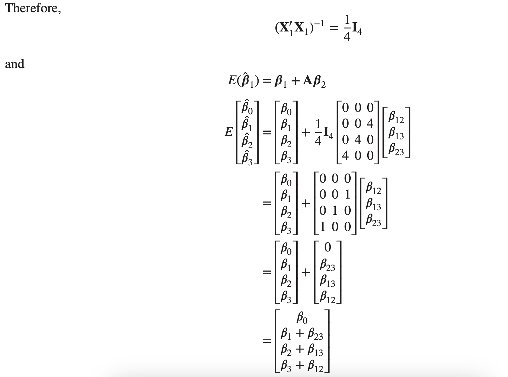
The interpretation of this is that each of the main effects is aliased with one of the two-factor interactions.

While this is a very simple example, the method is very general and can be applied to much more complex designs.

8.6 Resolution III Designs

• The sequential use of fractional factorial designs is very useful, often leading to great economy and efficiency in experimentation.

• This application of fractional factorials occurs frequently in situations of pure factor screening; that is, there are relatively many factors but only a few of them are expected to be important. Resolution III designs can be very useful in these situations.

---

• It is possible to construct resolution III designs for investigating up to $k=N-1$ factors in only $N$ runs, where $N$ is a multiple of 4.

• These designs are frequently useful in industrial experimentation.

• Important designs are 4 runs for up to 3 factors, 8 runs for up to 7 factors, and 16 runs for up to 15 factors.

• If $k=N-1$, the fractional factorial design is said to be saturated.

• A very useful saturated fractional factorial is a design for studying seven factors in eight runs, that is, the $2_{\text{III }}{}^{7-4}$ design. This design is a one-sixteenth fraction of the $2^7$.

---

• $2_{\text{III }}{}^{7-4}$ design may be constructed as follows:

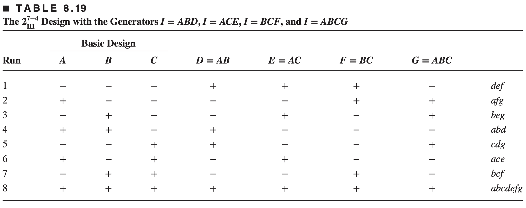
• The generators for this design are $I=ABD,I=$ $ACE,I=BCF$, and $I=ABCG$.

---

• The complete defining relation for this design is obtained by multiplying the four generators $ABD,ACE,BCF$, and $ABCG$ together two at a time, three at a time, and four at a time, yielding $$\begin{array}{rl}& I=ABD=ACE=BCF=ABCG=BCDE=ACDF=CDG\\ & =ABEF=BEG=AFG=DEF=ADEG=CEFG=BDFG\\ & =ABCDEFG\end{array}$$

• To find the aliases of any effect, simply multiply the effect by each word in the defining relation. For example, the aliases of $B$ are $$\begin{array}{rl}& B=AD=ABCE=CF=ACG=CDE=ABCDF=BCDG=\\ & AEF=EG=ABFG=BDEF=ABDEG=BCEFG=DFG\\ & =ACDEFG\end{array}$$

---

• This design is a one-sixteenth fraction, and because the signs chosen for the generators are positive, this is the principal fraction.

• Any one of the 16 different $2_{\text{III }}^{7-4}$ designs in this family could be constructed by using the generators with one of the 16 possible arrangements of signs in $I=\pm ABD,I=\pm ACE,I=\pm BCF,I=\pm ABCG$.

• The seven degrees of freedom in this design may be used to estimate the seven main effects.

---

• Each of these effects has 15 aliases; however, if we assume that three-factor and higher interactions are negligible, then considerable simplification in the alias structure results.

• Making this assumption, each of the linear combinations associated with the seven main effects in this design actually estimates the main effect and three two-factor interactions:

---

---

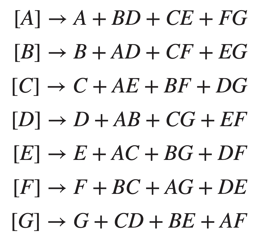
• These aliases can be found in Appendix Table $X(h)$.

• The saturated design $2_{\text{III }}^{7-4}$ can be used to obtain resolution III designs for studying fewer than seven factors in eight runs.

• For example, to generate a design for six factors in eight runs, simply drop any one column for example column G. This produces the design shown below

---

---

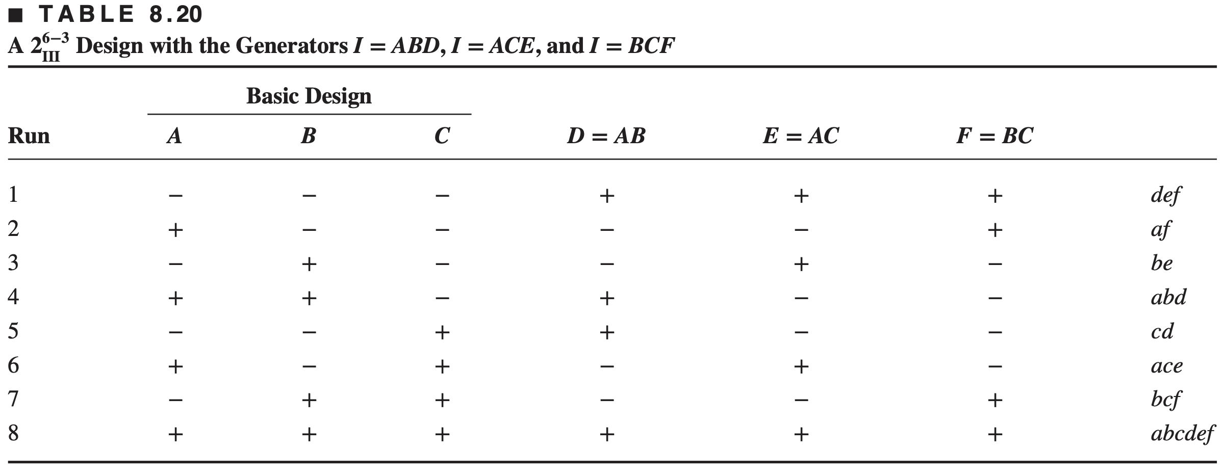
• It is easy to verify that this design is also of resolution III; in fact, it is a $2_{III}{}^{6-3}$, or a one eighth fraction, of the $2^6$ design.

• The defining relation for the $2_{III}^{6-3}$ design is equal with any words containing the letter $G$ deleted.

• Thus, the defining relation for our new design is $$I=ABD=ACE=BCF=BCDE=ACDF=ABEF=DEF$$

---

• It is also possible to obtain a resolution III design for studying up to 15 factors in 16 runs.

• This saturated $2_{III}^{15-11}$ design can be generated by first writing down the 16 treatment combinations associated with a $2^4$ design in $A,B,C$, and $D$ and then equating 11 new factors with the two-, three-, and four-factor interactions of the original four.

• In this design, each of the 15 main effects is aliased with seven two-factor interactions.

• A similar procedure can be used for the $2_{III}{}^{31-26}$ design, which allows up to 31 factors to be studied in 32 runs.

8.6.2 Fold Over of Resolution III Fractions to Separate Aliased Effects

Fold Over of Resolution III

• By combining fractional factorial designs in which certain signs are switched, we can systematically isolate effects of potential interest.

• This type of sequential experiment is called a fold over of the original design

---

• Consider the $2_{III}{}^{7-4}$ design in Table 8.19. Suppose that a second fractional design with the signs reversed in the column for factor $D$ is also run.

Run	A	B	C	D=-AB	E=AC	F=BC	G=ABC	Treat. comb.
1	-	-	-	+ -	+	+	-	ef
2	+	-	-	- +	-	+	+	afg
3	-	+	-	- +	+	-	+	beg
4	-	-	+	+ -	-	-	+	cg
5	+	+	-	+ -	-	-	-	ab
6	+	-	+	- +	+	-	-	ace
7	-	+	+	- +	-	+	-	bcf
8	+	+	+	+ -	+	+	+	abcefg

---

• The effects that may be estimated from this second fraction are: $$\begin{array}{rl}& [A{]}^{\prime }\to A-BD+CE+FG\\ & [B{]}^{\prime }\to B-AD+CF+EG\\ & [C{]}^{\prime }\to C+AE+BF-DG\\ & [D{]}^{\prime }\to D-AB-CG-EF\\ & [-D{]}^{\prime }\to -D+AB+CG+EF\\ & [E{]}^{\prime }\to E+AC+BG-DF\\ & [F{]}^{\prime }\to F+BC+AG-DE\\ & [G{]}^{\prime }\to G-CD+BE+AF\end{array}$$

---

Now from the two linear combinations of effects $\frac{1}{2}([\mathrm{i}]+[\mathrm{i}{]}^{\prime })$ and $\frac{1}{2}([\mathrm{i}]-[\mathrm{i}{]}^{\prime })$ we obtain

---

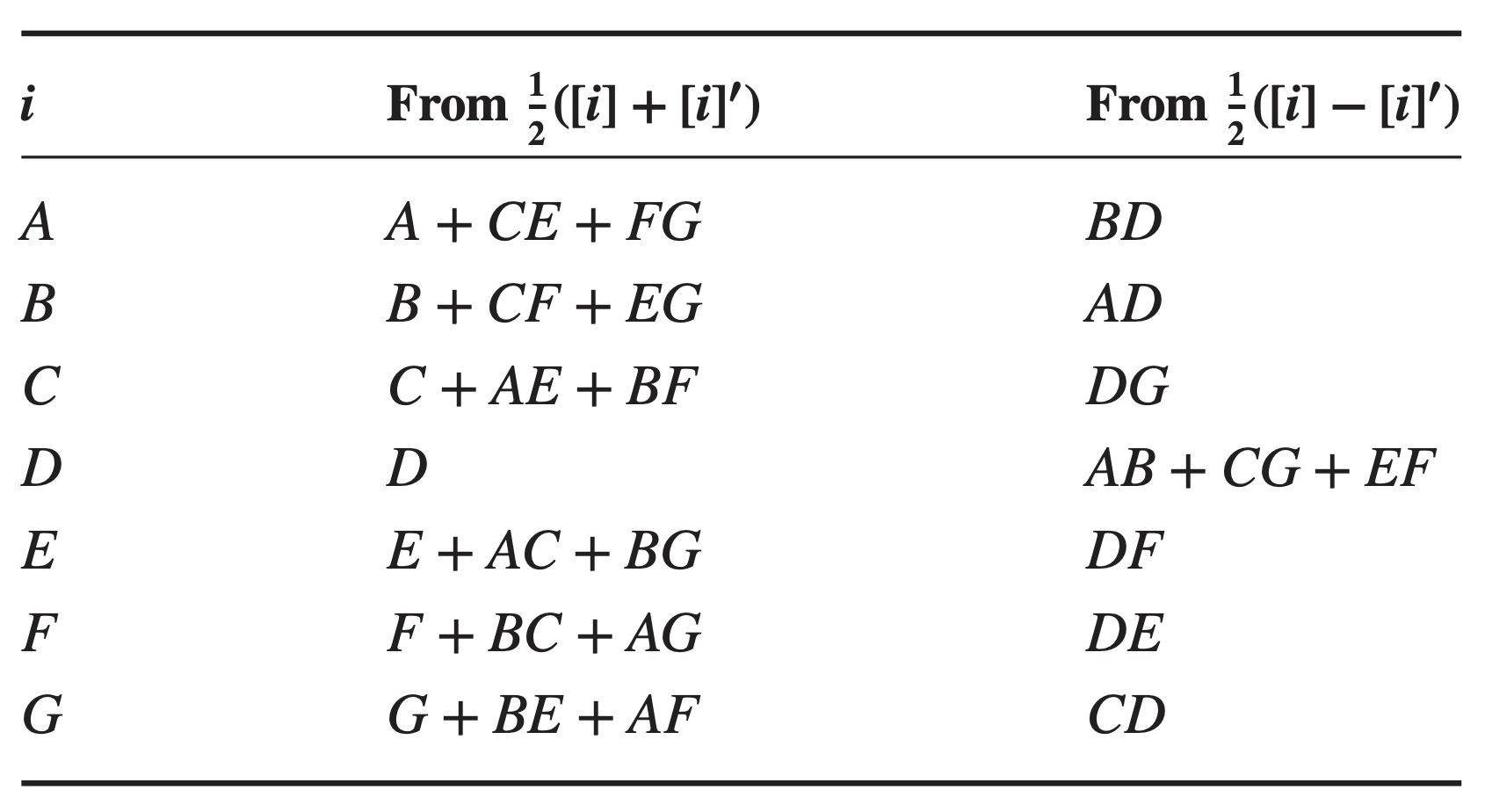
Thus, we have isolated the main effect of $D$ and all of its two-factor interactions.

In general, if we add to a fractional design of resolution III or higher a further fraction with the signs of a single factor reversed, then the combined design will provide estimates of the main effect of that factor and all of its two-factor interactions.

This is sometimes called a single-factor fold over.

---

Now suppose we add to a resolution III fractional a second fraction in which the signs for all the factors are reversed.

This type of fold over (sometimes called a full fold over or a reflection) breaks the alias links between all main effects and their two-factor interactions.

That is, we may use the combined design to estimate all of the main effects clear of any two factor interactions.

Example 8.7: Eye Focus Time Experiment

(illustrates a fold-over technique)

A human performance analyst is conducting an experiment to study eye focus time and has built an apparatus in which several factors can be controlled during the test.

The factors he initially regards as important are acuity or sharpness of vision ($A$), distance from target to eye ($B$), target shape ($C$), illumination level ($D$), target size ($E$), target density ($F$), and subject ($G$).

---

Two levels of each factor are considered. He suspects that only a few of these seven factors are of major importance and that high-order interactions between the factors can be neglected.

On the basis of this assumption, the analyst decides to run a screening experiment to identify the most important factors and then to concentrate further study on those.

To screen these seven factors, he runs the treatment combinations from the $2_{III}^{7-4}$ design.

---

After running the treatment combinations in random order the focus times in milliseconds are shown below

---

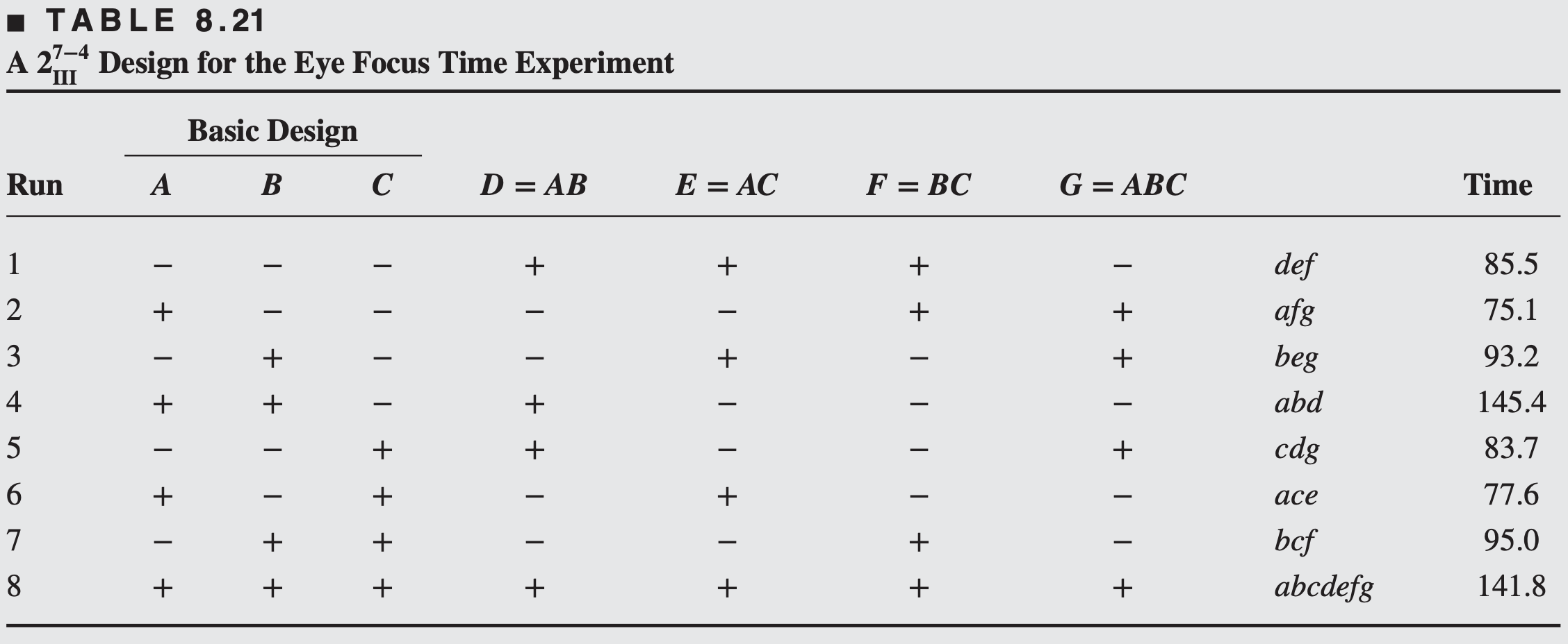
• Seven main effects and their aliases may be estimated from these data. From Equation 8.2, we see that the effects and their aliases are

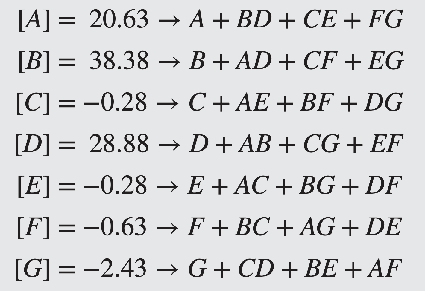
• For example, the estimate of main effect of $A$ and its aliases is $$\begin{array}{rl}[A]=\frac{1}{4}& (-85.5+75.1-93.2+145.4-83.7\\ & +77.6-95.0+141.8)=20.63\end{array}$$

---

The three largest effects are $[A]$, $[B]$, and $[D]$.

• Could be the main effects of $A,B$, and $D$ are all significant.

• Or $A,B$, and the $AB$ interaction

• Or perhaps $B,D$, and the $BD$ interaction

• Or perhaps $A,D$, and the $AD$ interaction

---

To separate the main effects and the two-factor interactions, the full fold-over technique is used, and a second fraction is run with all the signs reversed.

---

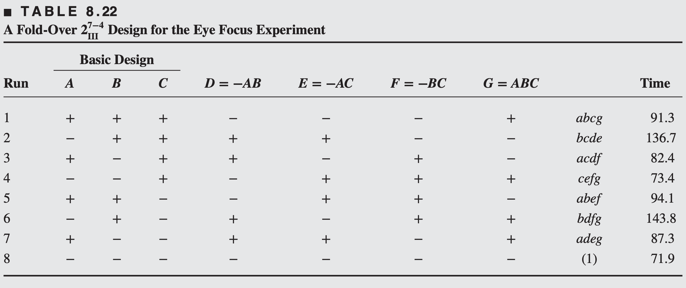
Notice that when we construct a full fold over of a resolution III design, we (in effect) change the signs on the generators that have an odd number of letters. The effects estimated by this fraction are

---

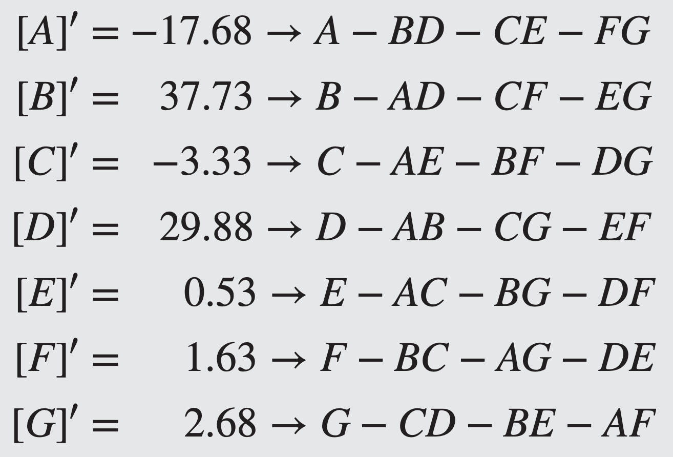
By combining this second fraction with the original one, we obtain the following estimates of the effects:

---

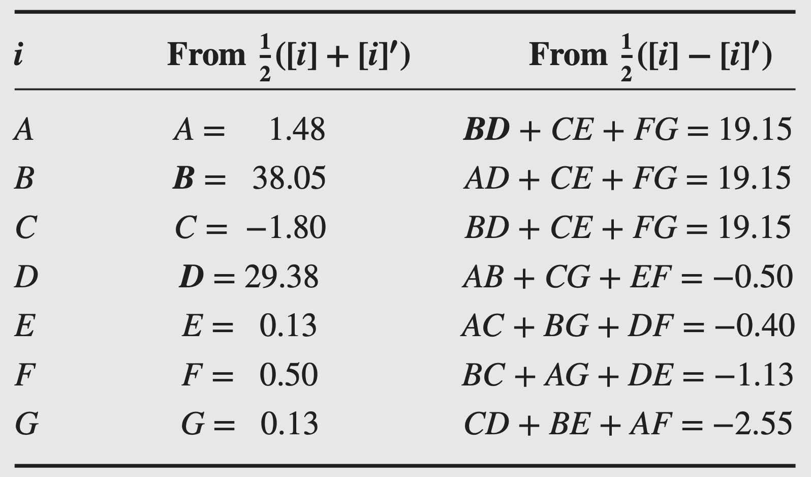
The two largest effects are $B$ and $D$. Furthermore, the third largest effect is $BD+CE+FG$, so it seems reasonable to attribute this to the $BD$ interaction.

The experimenter used the two factors distance $(B)$ and illumination level $(D)$ in subsequent experiments with the other factors $A,C,E$, and $F$ at standard settings and verified the results obtained here.

Defining Relation for a Fold-Over Design

It is often of interest to know the defining relation for the combined fractional factorial designs via fold over design.

Each separate fraction will have $L+U$ words used as generators: $L$ words of like sign and $U$ words of unlike sign.

The combined design will have $L+U-1$ words used as generators.

---

These will be the $L$ words of like sign and the $U-1$ words consisting of independent even products of the words of unlike sign.

Even products are words taken two at a time, four at a time, and so forth.

To illustrate this procedure, consider the design in Example 8.7. For the first fraction, the generators are $$I=ABD,I=ACE,I=BCF\text{, and }I=ABCG$$

---

and for the second fraction, they are $$I=-ABD,I=-ACE,I=-BCF\text{, and }I=ABCG$$ Notice that in the second fraction $L+U=1+3=4$. The combined design will have $I=ABCG$ (the like sign word) as a generator and two words that are independent even products of the words of unlike sign.

For example, take $I=ABD$ and $I=ACE$; then $I=(ABD)(ACE)=BCDE$ is a generator of the combined design.

---

Also, take $I=ABD$ and $I=BCF$; then $I=(ABD)(BCF)=ACDF$ is a generator of the combined design.

The complete defining relation for the combined design is $I=ABCG=BCDE=ACDF=ADEG=BDFG=ABEF=CEFG$

Blocking in a Fold-Over Design

Usually a fold-over design is conducted in two distinct time periods.

Following the initial fraction, some time usually elapses while the data are analyzed and the fold-over runs are planned.

Then the second set of runs is made, often on a different day, or different shift, or using different operating personnel, or perhaps material from a different source

---

This leads to a situation where blocking to eliminate potential nuisance effects between the two time periods is of interest.

To illustrate, consider the fold-over experiment in Example 8.7. In the initial group of eight runs the generators are $D=AB,E=AC,F=BC$, and $G=ABC$.

In the fold-over set of runs, the signs are changed on three of the generators so that $D=-AB,E=-AC,$ and $F=-BC$.

---

Thus, in the first group of eight runs the signs on the effects $ABD,ACE$, and $BCF$ are positive, and in the second group of eight runs the signs on $ABD,ACE$, and $BCF$ are negative; therefore, these effects are confounded with blocks.

Actually, there is a single-degree-of-freedom alias chain confounded with blocks and the effects in this alias chain may be found by multiplying any one of the effects $ABD,ACE$, and $BCF$ through the defining relation for the design. This yields

$ABD=CDG=ACE=BCF=BEG=AFG=DEF=ABCDEFG$ as the complete set of effects that are confounded with blocks.

In general, a completed fold over experiment will always form two blocks with the effects whose signs are positive in one block and negative in the other (and their aliases) confounded with blocks.

---

Summary of 8.6.2

• Fold over design: Sequential assembly of fractions to separate aliased effects

• Switching the signs in one column provides estimates of that factor and all of its two-factor interactions - called single-factor fold-over

• Switching the signs in all columns dealiases all main effects from their two factor interaction alias chains - called a full fold-over

• Defining relation for a fold-over

• Be careful - these rules only work for Resolution III designs

• There are other rules for Resolution IV designs, and other methods for adding runs to fractions to dealias effects of interest

8.6.3 Plackett-Burman designs

• These are a different class of resolution III design

• The fractional factorials we have considered so far are for $n=4,8,16,32,64$,–runs, which were the power of 2 , e.g. $2^2,2^3,2^4$, etc.

• In Plackett-Burman designs, the number of runs, $N$, need only be a multiple of four (e.g. $N=4,8,12,16,20,24,28,32,36,40,\dots$)

• The designs where $N=12,20,24$, etc. are called nongeometric Plackett-Burman designs

• Because these designs cannot be represented as cubes, they are sometimes called nongeometric designs

---

The following table presents rows of plus and minus signs that are used to construct the Plackett– Burman designs for N = 12, 20, 24, and 36.

---

The designs for $N$ = 12, 20, 24, and 36 are obtained by writing the appropriate row as a column.

A second column is then generated from this first one by moving the elements of the column down one position and placing the last element in the first position. A third column is produced from the second similarly, and the process is continued until column $k$ is generated. A row of minus signs is then added, completing the design.

---

The design for N = 12 runs and k = 11 factors is shown below

---

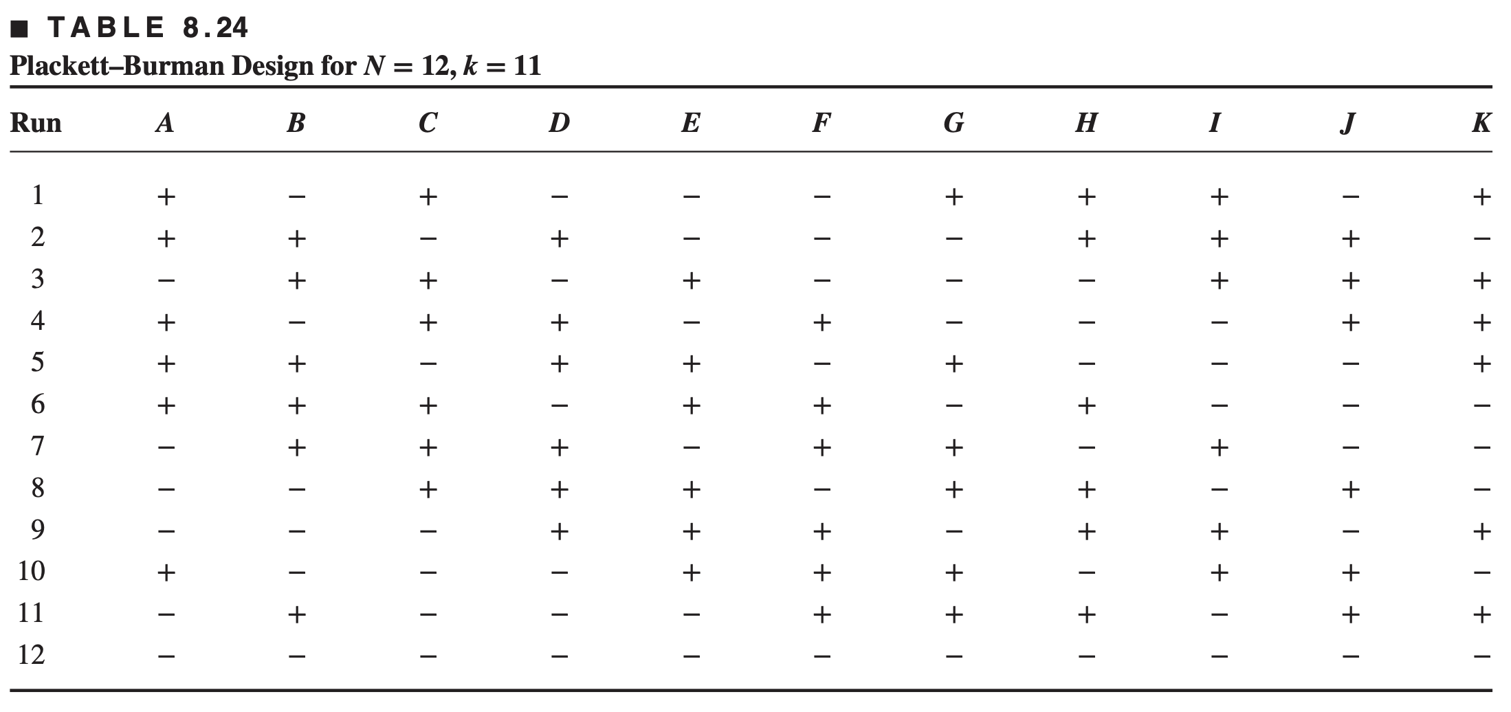
• The nongeometric Plackett-Burman designs for $N=12,20,24,28$, and 36 have complex alias structures.

• For example, in the 12 -run design every main effect is partially aliased with every two-factor interaction not involving itself.

  • For example, the $AB$ interaction is aliased with the nine main effects $C,D,\dots ,K$ and the $AC$ interaction is aliased with the nine main effects $B,D,\dots ,K$.

  • Furthermore, each main effect is partially aliased with 45 two-factor interactions. As an example, consider the aliases of the main effect of factor $A$: $$[A]=A-\frac{1}{3}BC-\frac{1}{3}BD-\frac{1}{3}BE+\frac{1}{3}BF+\cdots -\frac{1}{3}KL$$

---

Each one of the 45 two-factor interactions in the alias chain in weighed by the constant $\pm \frac{1}{3}$.

This weighting of the two-factor interactions occurs throughout the Plackett–Burman series of nongeometric designs.

In other Plackett–Burman designs, the constant will be different than $\pm \frac{1}{3}$.

8.7 Resolution IV and V Designs

A $2^{k-p}$ fractional factorial design is of resolution IV if the main effects are clear of two-factor interactions and some two-factor interactions are aliased with each other.

Thus, if three-factor and higher interactions are suppressed, the main effects may be estimated directly in a $2_{\mathrm{IV}}^{k-p}$ design. An example is the $2_{\mathrm{IV}}^{6-2}$ design in Table 8.10 . Furthermore, the two combined fractions of the $2_{\mathrm{III}}^{7-4}$ design in Example 8.7 yield a $2_{\mathrm{IV}}^{7-3}$ design.

Resolution IV designs are used extensively as screening experiments. The $2^{4-1}$ with eight runs and the 16 -run fractions with 6, 7, and 8 factors are very popular.

---

Any $2_{\text{IV }}^{k-p}$ design must contain at least $2k$ runs.

Resolution IV designs that contain exactly $2k$ runs are called minimal designs. Resolution IV designs may be obtained from resolution III designs by the process of fold over.

To fold over a $2_{III}^{k-p}$ design, simply add to the original fraction a second fraction with all the signs reversed.

Then the plus signs in the identity column $I$ in the first fraction could be switched in the second fraction, and a $(k+1)$st factor could be associated with this column. The result is a $2_{IV}{}^{k+1-p}$ fractional factorial design.

The process is demonstrated below for the $2_{III}^{3-1}$ design.

---

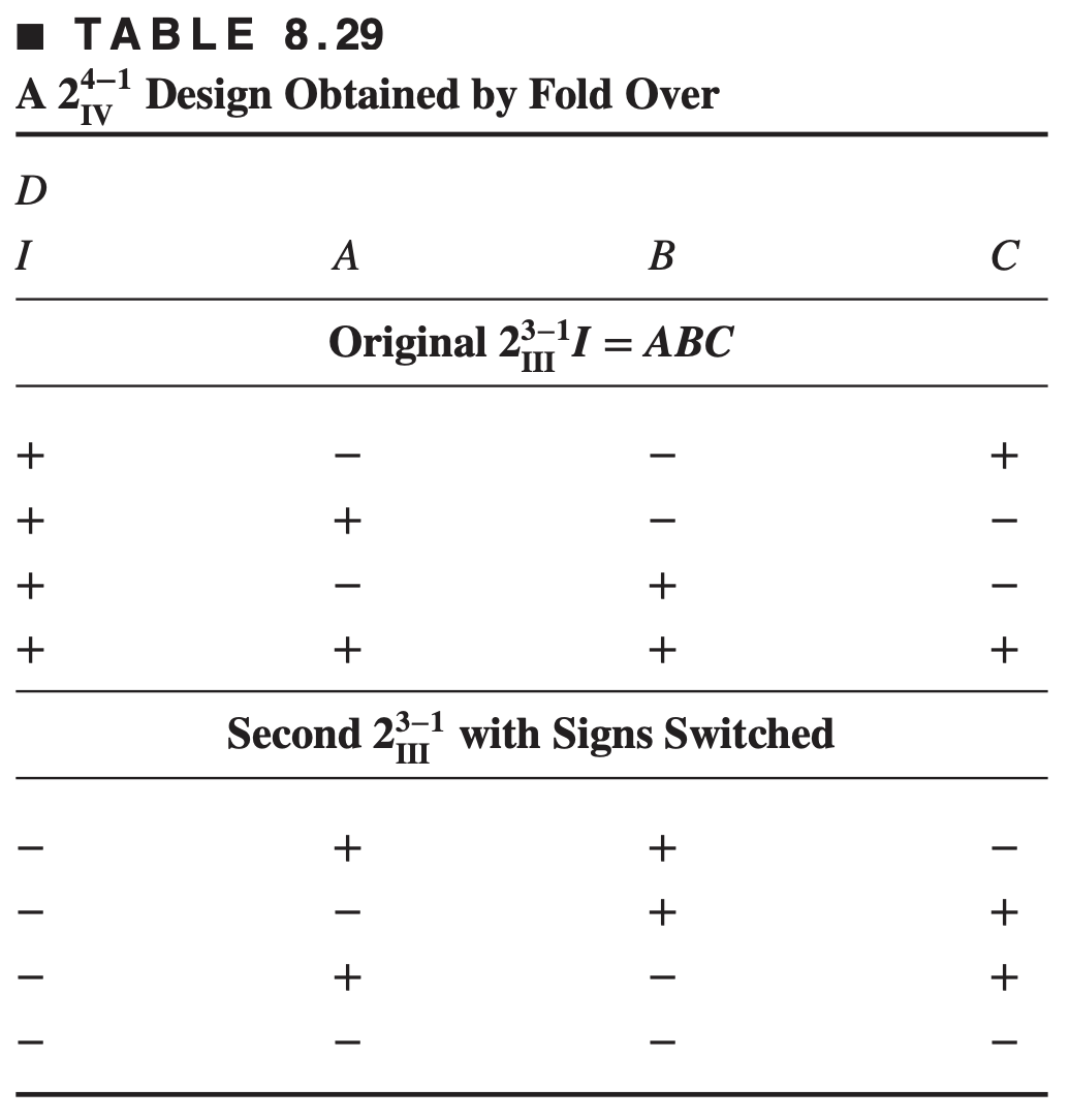
It is easy to verify that the resulting design is a design with defining relation $I=ABCD$

---

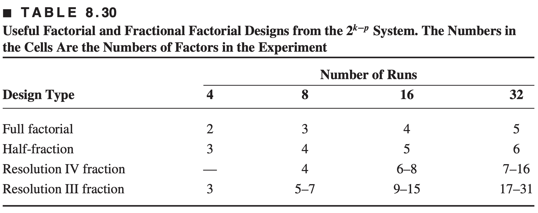
Table 8.30 provides a convenient summary of $2^{k-p}$ fractional factorial designs with $N$ = 4, 8, 16, and 32 runs.

Sequential Experimentation with Resolution IV Designs

Because resolution $IV$ designs are used as screening experiments, it is not unusual to find that upon conducting and analyzing the original experiment, additional experimentation is necessary to completely resolve all of the effects.

It is possible to fold over resolution IV designs to separate two-factor interactions that are aliased with each other.

---

An experimenter may have several objectives in folding over a resolution IV design, such as

1. Breaking as many two-factor interaction alias chains as possible,

2. Breaking the two-factor interactions on a specific alias chain, or

3. Breaking the two-factor interaction aliases involving a specific factor

---

However, one has to be careful in folding over a resolution IV design.

The full fold-over rule that we used for resolution III designs, simply run another fraction with all of the signs reversed, will not work for the resolution IV case. If this rule is applied to a resolution IV design, the result will be to produce exactly the same design with the runs in a different order. Try it! Use the $2_{IV}^{6-2}$ in Table 8.9 and see what happens when you reverse all of the signs in the test matrix.

The simplest way to fold over a resolution IV design is to switch the signs on a single variable of the original design matrix. This single-factor fold over allows all the two-factor interactions involving the factor whose signs are switched to be separated and accomplishes the third objective listed above

Example of single fold-over of Resolution IV

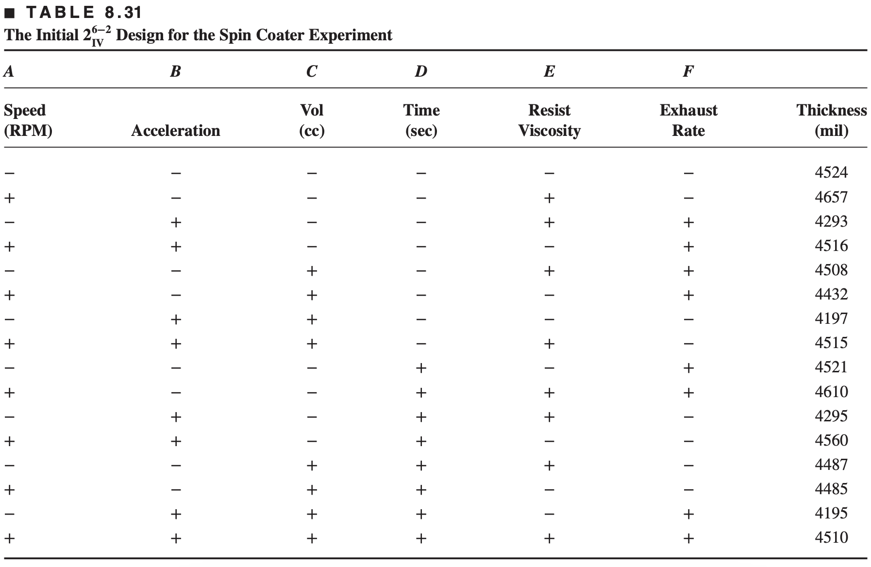
To illustrate how a single-factor fold over is accomplished for a resolution IV design, consider the following $2_{IV}^{6-2}$ design.

An experiment was conducted to study the effects of six factors on the thickness of photo-resist coating applied to a silicon wafer.

The design factors are $A=$ spin speed, $B=$ acceleration, $C=$ volume of resist applied, $D=$ spin time, $E=$ resist viscosity, and $F=$ exhaust rate.

---

---

Alias Structure for the $2_{IV}^{6-2}$ Design with $I=ABCE=BCDF=ADEF$ is

---

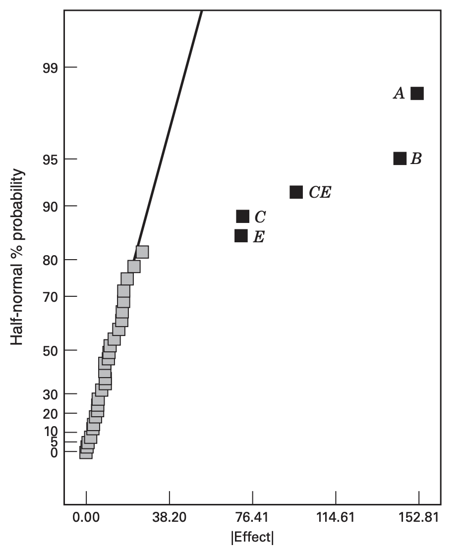
• The half-normal probability plot of the effects is

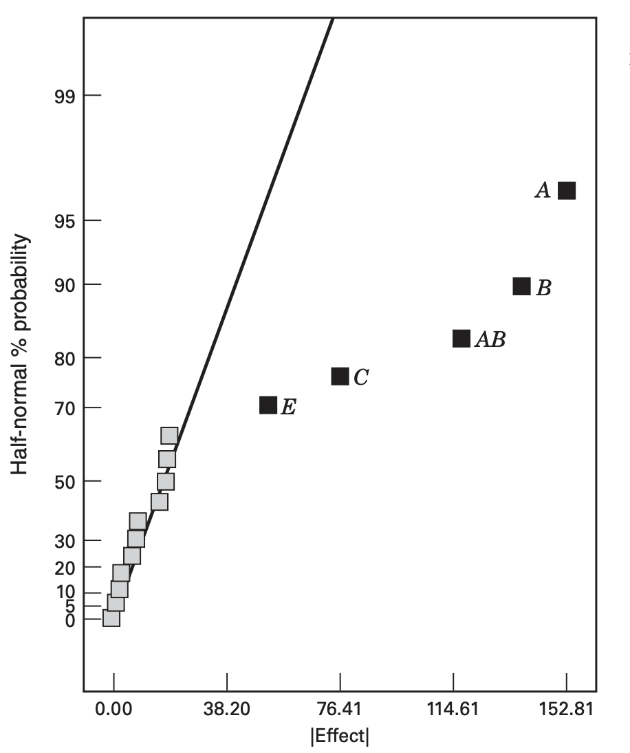
• The largest main effects are $A$, $B$, $C$, and $E$, and since these effects are aliased with three-factor or higher interactions, it is logical to assume that these are real effects.

• However, since $[AB]=AB+CE$ alias chain is also large. We do not know whether this is $AB$, $CE$, or both of the interaction effects.

---

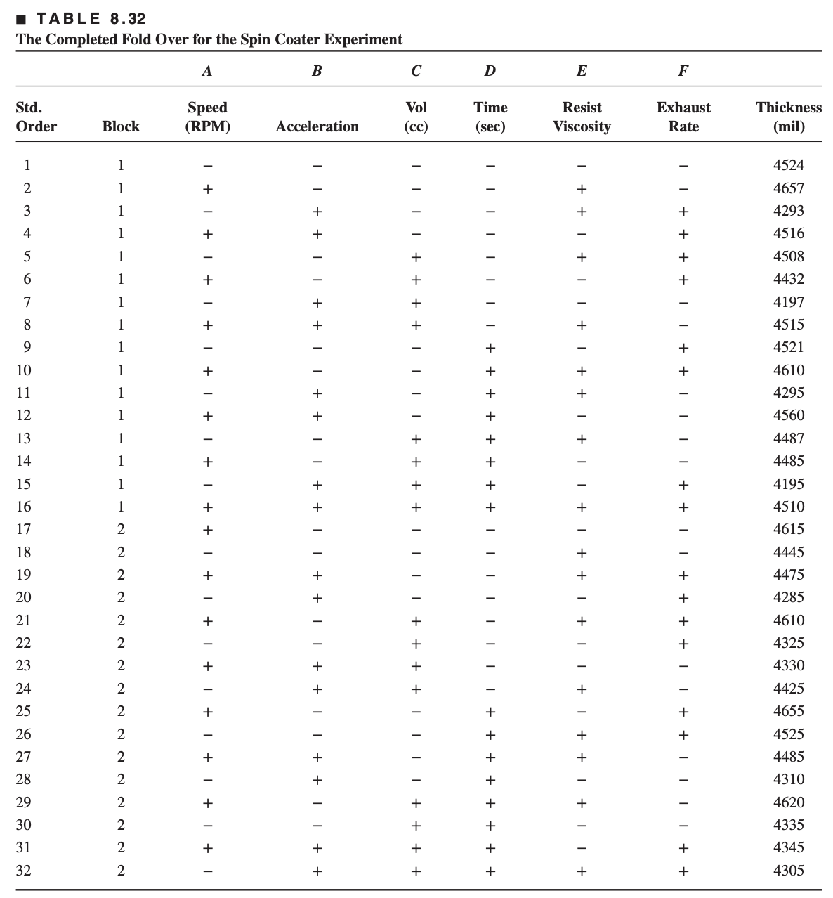
The fold-over design is constructed by setting up a new $2_{IV}{}^{6-2}$ fractional factorial design and changing the signs on factor $A$.

The complete design following the addition of the fold-over runs is shown below.

Notice that the runs have been assigned to two blocks; the runs from the initial $2_{IV}{}^{6-2}$ design are in block 1, and the fold-over runs are in block 2.

---

---

The effects that are estimated from the combined set of runs are (ignoring interactions involving three or more factors)

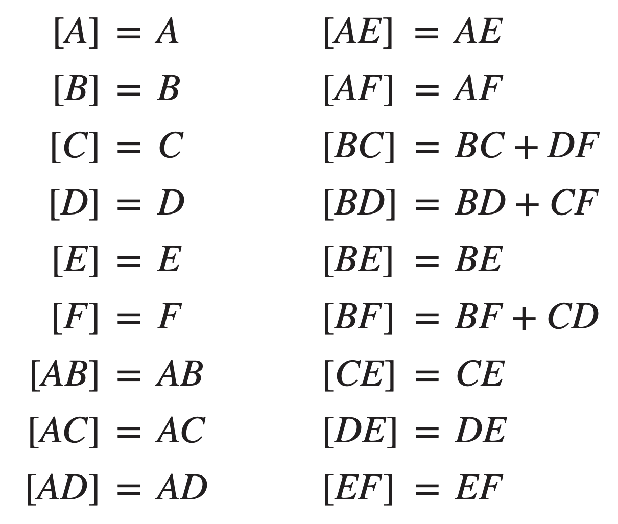
All of the two-factor interactions involving factor $A$ are now clear of other two factor interactions. Also, $AB$ is no longer aliased with $CE$.

---

The half-normal probability plot of the effects from the combined design clearly shows the $CE$ interaction is significant.

---

The generators for the original fractions are $E=ABC$ and $F=BCD$, and because we changed the signs in column A to create the fold over, the generators for the second group of 16 runs are $E=-ABC$ and $F=BCD$.

Since there is only one word of like sign $(L=1$, $U=1$ ) and the combined design has only one generator, the generator for the combined design is $F=BCD$.

Furthermore, since $ABCE$ is positive in block 1 and $ABCE$ is negative in block 2, $ABCE$ plus its alias $ADEF$ are confounded with blocks.

Full fold over of Resolution IV

• A full fold-over of a Resolution IV design is usually not necessary, and it’s potentially very inefficient.

• In the spin coater example, there were seven degrees of freedom available to estimate two-factor interaction alias chains.

• After adding the fold-over (16 more runs), there are only 12 degrees of freedom available for estimating two-factor interactions (16 new runs yields only five more degrees of freedom).

Resolution V Designs

Resolution $V$ designs are fractional factorials in which the main effects and the two-factor interactions do not have other main effects and two-factor interactions as their aliases.

Consequently, these are very powerful designs, allowing unique estimation of all main effects and two-factor interactions, provided of course that all interactions involving three or more factors are negligible.

The shortest word in the defining relation of a resolution $V$ design must have five letters.

The $2^{5-1}$ design with $I=ABCDE$ is perhaps the most widely used resolution $V$ design, permitting study of five factors and estimation of all five main effects and all 10 two factor interactions in only 16 runs.

Generally, Resolution $V$ designs are large (at least 32 runs) for six or more factors